Create tornado bar-plots of the differences between two model runs.
e2ep_compare_runs_bar.RdCreate a tornado bar-plot diagram of the differences in either annual average masses of ecology model varibles, or annual fishery catches, between two different runs of the StrathE2E model, referred to as baseline and sceanrio runs.
Usage
e2ep_compare_runs_bar(
  selection = "AAM",
  model1 = NA,
  use.saved1 = FALSE,
  results1,
  model2 = NA,
  use.saved2 = FALSE,
  results2,
  log.pc = "PC",
  zone = "W",
  bpmin = (-50),
  bpmax = (+50),
  maintitle = ""
)
Arguments
- selection
Text string from a list identifying which type of data are to be plotted. Select from: "AAM", "CATCH", corresponding to annual average mass data, and catch data respectively (default = "AAM"). Remember to include the phrase within "" quotes.
- model1
R-list object defining the baseline model configuration compiled by the e2ep_read() function.
- use.saved1
Logical. If TRUE then use baseline data from a prior user-defined run held as csv files data in the current results folder (default=FALSE).
- results1
R-list object of baseline model output generated by the e2ep_run() (default=NULL).
- model2
R-list object defining the scenario model configuration compiled by the e2ep_read() function.
- use.saved2
Logical. If TRUE then use scenario data from a prior user-defined run held as csv files data in the current results folder (default=FALSE).
- results2
R-list object of scenario model output generated by the e2ep_run() (default=NULL).
- log.pc
Value="LG" for data to be plotted on a log10 scale, value = "PC" for data to be plotted on a percentage difference scale (default = "PC").
- zone
Value = "O" for offshore, "I" for inshore, or "W" for whole model domain (all upper case) (default = "W").
- bpmin
Axis minimum for plot - i.e. the maximum NEGATIVE value of (scenario-baseline). Default = -50, given log.pc="PC" (percentage differences). Needs to be reset to e.g. -0.3 if log.pc="LG" (log scale).
- bpmax
Axis maximum for plot - i.e. the maximum POSITIVE value of (scenario-baseline). Default = +50, given log.pc="PC" (percentage differences). Needs to be reset to e.g. +0.3 if log.pc="LG" (log scale).
- maintitle
A optional descriptive text field (in quotes) to be added above the plot. Keep to 45 characters including spaces (default="").
Value
List object comprising two dataframes of the displayed data, graphical display in a new graphics window.
Details
A tornado plot is a horizontal barplot which shows the difference between baseline and sceanrio runs. Bars to the right indicate scenario values greater than the baseline, bars to the left indicate scenario values less than baseline. In this function the difference between scenario and baseline data is calculated as either ((scenario - baseline)/baseline) and plotted on a linear (percentage) scale, or (scenario/baseline) and plotted on a log10 scale. In both cases, zero represents scenario = baseline.
The choice of whether to plot data on the masses of ecosystem components, or fishery catches, is determined by an argument setting in the function call. In either case two panels of tornado diagrams are plotted. In the case of mass data, the panels show data on water column components of the ecoststem (upper panel) and seabed components of the system (lower panel). In the case of catch data, the upper panel shows landings, the lower shows discards. For mass data and landings, positive values (scenario > baseline) are indicated by green bars to the right, negative values (scenario < baseline) by red bars to the left. For discards, positive values are in black, negative in grey. For any bars extending outsided the selected plotting range, the numeric value is displayed inside the relevant bar.
The function accepts data from either saved csv files created by the e2ep_run() function, or directly from e2ep_run() results objects. The relevant csv files are: /results/Modelname/Variantname/ZONE_model_anav_biomass-*.csv where ZONE is INSHORE, OFFSHORE or WHOLEDOMAIN and * represents the model run identifier (model.ident) embedded in the R-list object created by the e2ep_read() function.
In addition to generating graphics output the function returns a list object of the data presented in the plot. The object comprises two dataframes (changewater and changeseabed where annual average mass data are selected; changeland and changedisc where catch data are selected). The first column in each dataframe is the proportional difference expressed on a log10 scale, the second column as a percentage.
Examples
# Load the 2011-2019 version of the internal Barents Sea model and run for 1 year
m1 <- e2ep_read("Barents_Sea", "2011-2019",model.ident="11-19")
#> Current working directory is...
#> 'C:/Users/jackl/OneDrive - University of Strathclyde/Documents/StrathE2E/strath-e-2-e-polar-webdev/docs/reference'
#> No 'results.path' specified so any csv data requested
#> will be directed to/from the temporary directory...
#> 'C:\Users\jackl\AppData\Local\Temp\RtmpSgdWsc'
#>
#> Model setup and parameters gathered from ...
#> StrathE2E2 package folder
#> Model results will be directed to/from ...
#> 'C:\Users\jackl\AppData\Local\Temp\RtmpSgdWsc/Barents_Sea/2011-2019/'
r1 <-e2ep_run(m1,nyears=1)
# Load the 2011-2019 version of the internal Barents Sea model, modify, and run for 1 year
m2 <- e2ep_read("Barents_Sea", "2011-2019",model.ident="plus1C")
#> Current working directory is...
#> 'C:/Users/jackl/OneDrive - University of Strathclyde/Documents/StrathE2E/strath-e-2-e-polar-webdev/docs/reference'
#> No 'results.path' specified so any csv data requested
#> will be directed to/from the temporary directory...
#> 'C:\Users\jackl\AppData\Local\Temp\RtmpSgdWsc'
#>
#> Model setup and parameters gathered from ...
#> StrathE2E2 package folder
#> Model results will be directed to/from ...
#> 'C:\Users\jackl\AppData\Local\Temp\RtmpSgdWsc/Barents_Sea/2011-2019/'
m2$data$physics.drivers$so_temp<-m2$data$physics.drivers$so_temp+1
# 1-degC added to offshore zone upper layer temperatures
r2 <-e2ep_run(m2,nyears=1)
# Compare the annual average mass in 2011-2019 (as the baseline case) with "plus1C"
# (as the scenario case):
mdiff_results1 <- e2ep_compare_runs_bar(selection="AAM",
model1=NA, use.saved1=FALSE, results1=r1,
model2=NA, use.saved2=FALSE, results2=r2,
log.pc="PC", zone="W",
bpmin=(-50),bpmax=(+50),
maintitle="2011-2019 compared with 1C warmer")
#> [1] "Using baseline data held in memory from an existing model run"
#> [1] "Using scenario data held in memory from an existing model run"
 mdiff_results1
#> $changewater
#> LG PC
#> Ice detritus -2.650772e-03 -0.6085037701
#> Ice and snow ammonia 6.256033e-06 0.0014405151
#> Ice and snow nitrate 8.644515e-03 2.0104151940
#> Ice algae 1.842223e-03 0.4250885665
#> Suspended bacteria & detritus -4.747955e-03 -1.0873027597
#> Water column ammonia 2.552820e-03 0.5895394160
#> Water column nitrate -4.004851e-04 -0.0921725907
#> Macrophytes -4.632523e-05 -0.0106662105
#> Phytoplankton 4.184807e-04 0.0964051835
#> Benthic susp/dep feeder larvae -5.473086e-03 -1.2523170005
#> Omnivorous zooplankton 1.094415e-03 0.2523161881
#> Benthic carn/scav feeder larvae -1.721327e-03 -0.3955658031
#> Carnivorous zooplankton 2.903137e-03 0.6707112713
#> Plantiv. fish adults+larvae 8.717686e-04 0.2009337346
#> Migratory fish 6.351458e-05 0.0146258430
#> Demersal fish adults+larvae 1.767584e-03 0.4078306539
#> Birds 4.600663e-05 0.0105939784
#> Pinnipeds 4.202251e-05 0.0096765082
#> Cetaceans 3.369933e-05 0.0077598592
#> Maritime mammals 3.728198e-06 0.0008584529
#>
#> $changeseabed
#> LG PC
#> Fishery discards & offal 6.886097e-04 0.158684003
#> Corpses -3.963611e-03 -0.908502995
#> Sediment bacteria & detritus -1.319411e-05 -0.003038011
#> Macrophyte debris -2.608425e-05 -0.006005941
#> Porewater ammonia -1.275714e-03 -0.293313091
#> Porewater nitrate -2.339786e-04 -0.053861051
#> Benthic susp/dep feeders -1.421083e-03 -0.326681697
#> Benthic carn/scav feeders -1.107981e-03 -0.254796881
#>
# Compare the annual catch in 2011-2019 (as the baseline case) with "plus1C"
# (as the scenario case):
mdiff_results2 <- e2ep_compare_runs_bar(selection="CATCH",
model1=NA, use.saved1=FALSE, results1=r1,
model2=NA, use.saved2=FALSE, results2=r2,
log.pc="LG", zone="W",
bpmin=(-0.9),bpmax=(+0.4),
maintitle="2011-2019 compared with 1C warmer")
#> [1] "Using baseline data held in memory from an existing model run"
#> [1] "Using scenario data held in memory from an existing model run"
mdiff_results1
#> $changewater
#> LG PC
#> Ice detritus -2.650772e-03 -0.6085037701
#> Ice and snow ammonia 6.256033e-06 0.0014405151
#> Ice and snow nitrate 8.644515e-03 2.0104151940
#> Ice algae 1.842223e-03 0.4250885665
#> Suspended bacteria & detritus -4.747955e-03 -1.0873027597
#> Water column ammonia 2.552820e-03 0.5895394160
#> Water column nitrate -4.004851e-04 -0.0921725907
#> Macrophytes -4.632523e-05 -0.0106662105
#> Phytoplankton 4.184807e-04 0.0964051835
#> Benthic susp/dep feeder larvae -5.473086e-03 -1.2523170005
#> Omnivorous zooplankton 1.094415e-03 0.2523161881
#> Benthic carn/scav feeder larvae -1.721327e-03 -0.3955658031
#> Carnivorous zooplankton 2.903137e-03 0.6707112713
#> Plantiv. fish adults+larvae 8.717686e-04 0.2009337346
#> Migratory fish 6.351458e-05 0.0146258430
#> Demersal fish adults+larvae 1.767584e-03 0.4078306539
#> Birds 4.600663e-05 0.0105939784
#> Pinnipeds 4.202251e-05 0.0096765082
#> Cetaceans 3.369933e-05 0.0077598592
#> Maritime mammals 3.728198e-06 0.0008584529
#>
#> $changeseabed
#> LG PC
#> Fishery discards & offal 6.886097e-04 0.158684003
#> Corpses -3.963611e-03 -0.908502995
#> Sediment bacteria & detritus -1.319411e-05 -0.003038011
#> Macrophyte debris -2.608425e-05 -0.006005941
#> Porewater ammonia -1.275714e-03 -0.293313091
#> Porewater nitrate -2.339786e-04 -0.053861051
#> Benthic susp/dep feeders -1.421083e-03 -0.326681697
#> Benthic carn/scav feeders -1.107981e-03 -0.254796881
#>
# Compare the annual catch in 2011-2019 (as the baseline case) with "plus1C"
# (as the scenario case):
mdiff_results2 <- e2ep_compare_runs_bar(selection="CATCH",
model1=NA, use.saved1=FALSE, results1=r1,
model2=NA, use.saved2=FALSE, results2=r2,
log.pc="LG", zone="W",
bpmin=(-0.9),bpmax=(+0.4),
maintitle="2011-2019 compared with 1C warmer")
#> [1] "Using baseline data held in memory from an existing model run"
#> [1] "Using scenario data held in memory from an existing model run"
 mdiff_results2
#> $changeland
#> LG PC
#> Macrophytes NA NA
#> Susp/dep feeding benthos -2.690540e-03 -0.617604737
#> Carn/scav feeding benthos -1.352099e-03 -0.310848174
#> Pelagic invertebrates 5.042981e-03 1.167957343
#> Planktivorous fish 8.832086e-04 0.203573221
#> Migratory fish 9.234968e-05 0.021266560
#> Non-quota demersal fish 1.522147e-03 0.351102220
#> Quota-limited demersal fish 1.527330e-03 0.352299755
#> Birds NA NA
#> Pinnipeds -2.755523e-03 -0.632474105
#> Cetaceans 1.831582e-05 0.004217462
#>
#> $changedisc
#> LG PC
#> Macrophytes NA NA
#> Susp/dep feeding benthos NA NA
#> Carn/scav feeding benthos NA NA
#> Pelagic invertebrates NA NA
#> Planktivorous fish 9.370466e-04 0.215995885
#> Migratory fish 9.234968e-05 0.021266560
#> Non-quota demersal fish 1.615670e-03 0.372714643
#> Quota-limited demersal fish 1.627279e-03 0.375397779
#> Birds 4.686317e-05 0.010791226
#> Pinnipeds -7.745960e-05 -0.017834142
#> Cetaceans -4.384972e-06 -0.001009672
#>
# \donttest{
# Create a new scenario run from 2011-2019 case.
# Copy the 2011-2019 configuration into a new model object:
scen1_model <- m1
scen1_model$setup$model.ident <- "scenario1"
# Gear 4 (Beam_Trawl_BT1+BT2) activity rate rescaled to 0.5*baseline:
scen1_model$data$fleet.model$gear_mult[4] <- 0.5
scen1_results <- e2ep_run(scen1_model,nyears=20)
# Compare the annual average mass from the the 2011-2019 baseline with scenario1 data
mdiff_results3 <- e2ep_compare_runs_bar(selection="AAM",
model1=NA, use.saved1=FALSE, results1=r1,
model2=NA, use.saved2=FALSE, results2=scen1_results,
log.pc="PC", zone="W",
bpmin=(-30),bpmax=(+30),
maintitle="Beam Trawl activity reduced by half")
#> [1] "Using baseline data held in memory from an existing model run"
#> [1] "Using scenario data held in memory from an existing model run"
mdiff_results2
#> $changeland
#> LG PC
#> Macrophytes NA NA
#> Susp/dep feeding benthos -2.690540e-03 -0.617604737
#> Carn/scav feeding benthos -1.352099e-03 -0.310848174
#> Pelagic invertebrates 5.042981e-03 1.167957343
#> Planktivorous fish 8.832086e-04 0.203573221
#> Migratory fish 9.234968e-05 0.021266560
#> Non-quota demersal fish 1.522147e-03 0.351102220
#> Quota-limited demersal fish 1.527330e-03 0.352299755
#> Birds NA NA
#> Pinnipeds -2.755523e-03 -0.632474105
#> Cetaceans 1.831582e-05 0.004217462
#>
#> $changedisc
#> LG PC
#> Macrophytes NA NA
#> Susp/dep feeding benthos NA NA
#> Carn/scav feeding benthos NA NA
#> Pelagic invertebrates NA NA
#> Planktivorous fish 9.370466e-04 0.215995885
#> Migratory fish 9.234968e-05 0.021266560
#> Non-quota demersal fish 1.615670e-03 0.372714643
#> Quota-limited demersal fish 1.627279e-03 0.375397779
#> Birds 4.686317e-05 0.010791226
#> Pinnipeds -7.745960e-05 -0.017834142
#> Cetaceans -4.384972e-06 -0.001009672
#>
# \donttest{
# Create a new scenario run from 2011-2019 case.
# Copy the 2011-2019 configuration into a new model object:
scen1_model <- m1
scen1_model$setup$model.ident <- "scenario1"
# Gear 4 (Beam_Trawl_BT1+BT2) activity rate rescaled to 0.5*baseline:
scen1_model$data$fleet.model$gear_mult[4] <- 0.5
scen1_results <- e2ep_run(scen1_model,nyears=20)
# Compare the annual average mass from the the 2011-2019 baseline with scenario1 data
mdiff_results3 <- e2ep_compare_runs_bar(selection="AAM",
model1=NA, use.saved1=FALSE, results1=r1,
model2=NA, use.saved2=FALSE, results2=scen1_results,
log.pc="PC", zone="W",
bpmin=(-30),bpmax=(+30),
maintitle="Beam Trawl activity reduced by half")
#> [1] "Using baseline data held in memory from an existing model run"
#> [1] "Using scenario data held in memory from an existing model run"
 mdiff_results3
#> $changewater
#> LG PC
#> Ice detritus 6.206897e-04 0.1430212719
#> Ice and snow ammonia 8.625948e-02 21.9718131025
#> Ice and snow nitrate 1.622777e-02 3.8072712098
#> Ice algae 7.469177e-04 0.1721321242
#> Suspended bacteria & detritus -2.009770e-05 -0.0046275600
#> Water column ammonia -1.184446e-05 -0.0027272498
#> Water column nitrate -1.410535e-05 -0.0032478238
#> Macrophytes -2.519718e-06 -0.0005801848
#> Phytoplankton 9.584130e-05 0.0220707090
#> Benthic susp/dep feeder larvae 3.320278e-05 0.0076455147
#> Omnivorous zooplankton 8.235287e-06 0.0018962629
#> Benthic carn/scav feeder larvae -4.571517e-05 -0.0105257530
#> Carnivorous zooplankton 5.480589e-07 0.0001261953
#> Plantiv. fish adults+larvae -2.162673e-04 -0.0497849986
#> Migratory fish 5.539668e-06 0.0012755639
#> Demersal fish adults+larvae 8.059591e-04 0.1857512408
#> Birds 4.142971e-05 0.0095399978
#> Pinnipeds 2.073251e-04 0.0477497564
#> Cetaceans 1.047444e-04 0.0241211868
#> Maritime mammals 8.465569e-05 0.0194945933
#>
#> $changeseabed
#> LG PC
#> Fishery discards & offal -1.329361e-03 -3.056287e-01
#> Corpses -2.486920e-05 -5.726181e-03
#> Sediment bacteria & detritus -4.029302e-08 -9.277811e-06
#> Macrophyte debris -4.375714e-05 -1.007495e-02
#> Porewater ammonia 1.425890e-05 3.283287e-03
#> Porewater nitrate -1.558308e-05 -3.588073e-03
#> Benthic susp/dep feeders -6.859381e-06 -1.579418e-03
#> Benthic carn/scav feeders -1.492191e-05 -3.435838e-03
#>
# }
# \donttest{
# Create a second sceanario from the 2011-2019 case, this time saving the results to a file;
# csv output to temporary folder since results.path was not set in e2ep_read() when creating m1.
# Copy the baseline configuration into a new model object:
scen2_model <- m1
scen2_model$setup$model.ident <- "scenario2"
# Gear 1 (Pelagic_Trawl+Seine) activity rate rescaled to 0.5*baseline:
scen2_model$data$fleet.model$gear_mult[1] <- 0.5
scen2_results <- e2ep_run(scen2_model,nyears=20, csv.output=TRUE)
# Compare the annual catches in the 2011-2019 base line with the Pelagic Trawl/seine scenario
mdiff_results4 <- e2ep_compare_runs_bar(selection="CATCH",
model1=NA, use.saved1=FALSE, results1=r1,
model2=scen2_model,use.saved2=TRUE, results2=NA,
log.pc="LG", zone="W",
bpmin=(-0.4),bpmax=(+0.6),
maintitle="Pelagic Trawl/Seine activity reduced by half")
#> [1] "Using baseline data held in memory from an existing model run"
#> [1] "Using scenario data held in a csv files from a past model run"
mdiff_results3
#> $changewater
#> LG PC
#> Ice detritus 6.206897e-04 0.1430212719
#> Ice and snow ammonia 8.625948e-02 21.9718131025
#> Ice and snow nitrate 1.622777e-02 3.8072712098
#> Ice algae 7.469177e-04 0.1721321242
#> Suspended bacteria & detritus -2.009770e-05 -0.0046275600
#> Water column ammonia -1.184446e-05 -0.0027272498
#> Water column nitrate -1.410535e-05 -0.0032478238
#> Macrophytes -2.519718e-06 -0.0005801848
#> Phytoplankton 9.584130e-05 0.0220707090
#> Benthic susp/dep feeder larvae 3.320278e-05 0.0076455147
#> Omnivorous zooplankton 8.235287e-06 0.0018962629
#> Benthic carn/scav feeder larvae -4.571517e-05 -0.0105257530
#> Carnivorous zooplankton 5.480589e-07 0.0001261953
#> Plantiv. fish adults+larvae -2.162673e-04 -0.0497849986
#> Migratory fish 5.539668e-06 0.0012755639
#> Demersal fish adults+larvae 8.059591e-04 0.1857512408
#> Birds 4.142971e-05 0.0095399978
#> Pinnipeds 2.073251e-04 0.0477497564
#> Cetaceans 1.047444e-04 0.0241211868
#> Maritime mammals 8.465569e-05 0.0194945933
#>
#> $changeseabed
#> LG PC
#> Fishery discards & offal -1.329361e-03 -3.056287e-01
#> Corpses -2.486920e-05 -5.726181e-03
#> Sediment bacteria & detritus -4.029302e-08 -9.277811e-06
#> Macrophyte debris -4.375714e-05 -1.007495e-02
#> Porewater ammonia 1.425890e-05 3.283287e-03
#> Porewater nitrate -1.558308e-05 -3.588073e-03
#> Benthic susp/dep feeders -6.859381e-06 -1.579418e-03
#> Benthic carn/scav feeders -1.492191e-05 -3.435838e-03
#>
# }
# \donttest{
# Create a second sceanario from the 2011-2019 case, this time saving the results to a file;
# csv output to temporary folder since results.path was not set in e2ep_read() when creating m1.
# Copy the baseline configuration into a new model object:
scen2_model <- m1
scen2_model$setup$model.ident <- "scenario2"
# Gear 1 (Pelagic_Trawl+Seine) activity rate rescaled to 0.5*baseline:
scen2_model$data$fleet.model$gear_mult[1] <- 0.5
scen2_results <- e2ep_run(scen2_model,nyears=20, csv.output=TRUE)
# Compare the annual catches in the 2011-2019 base line with the Pelagic Trawl/seine scenario
mdiff_results4 <- e2ep_compare_runs_bar(selection="CATCH",
model1=NA, use.saved1=FALSE, results1=r1,
model2=scen2_model,use.saved2=TRUE, results2=NA,
log.pc="LG", zone="W",
bpmin=(-0.4),bpmax=(+0.6),
maintitle="Pelagic Trawl/Seine activity reduced by half")
#> [1] "Using baseline data held in memory from an existing model run"
#> [1] "Using scenario data held in a csv files from a past model run"
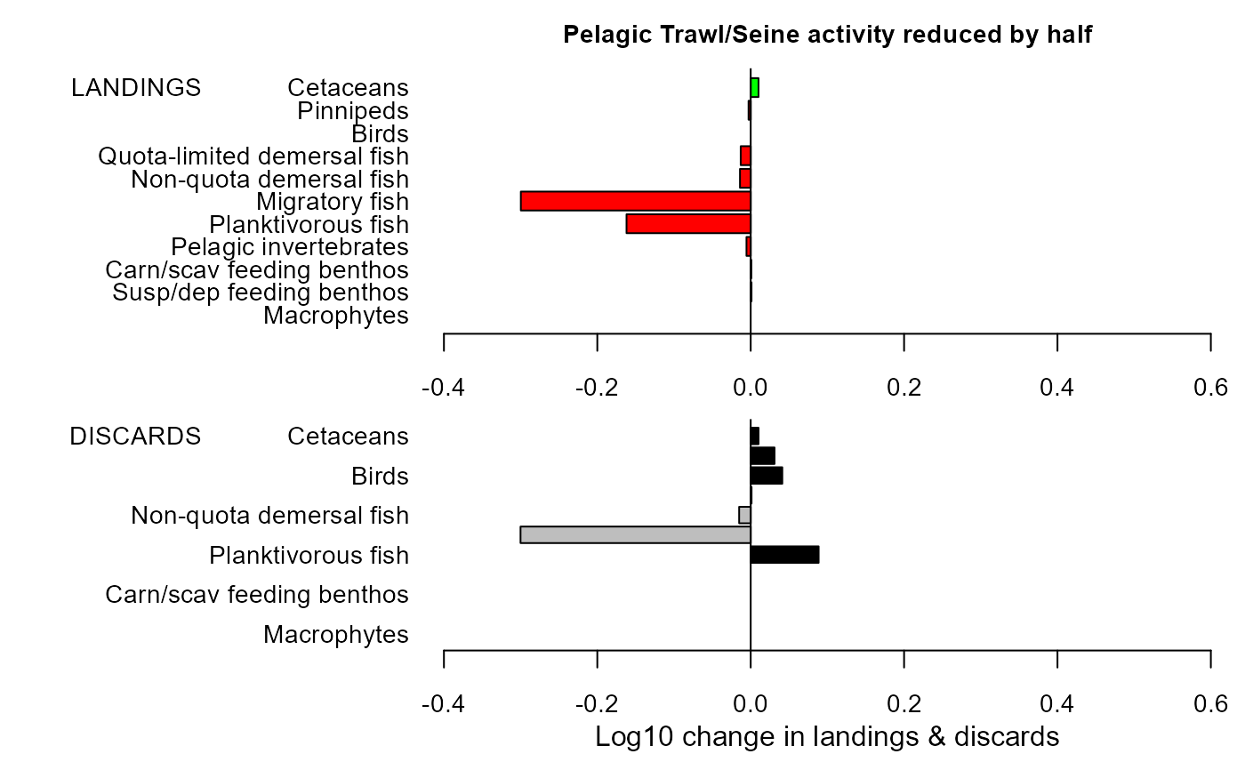 mdiff_results4
#> $changeland
#> LG PC
#> Macrophytes NA NA
#> Susp/dep feeding benthos 0.001056665 0.2436023
#> Carn/scav feeding benthos 0.000619318 0.1427050
#> Pelagic invertebrates -0.005491268 -1.2564511
#> Planktivorous fish -0.161913857 -31.1211094
#> Migratory fish -0.299716097 -49.8485027
#> Non-quota demersal fish -0.013951103 -3.1613120
#> Quota-limited demersal fish -0.013026904 -2.9550153
#> Birds NA NA
#> Pinnipeds -0.002786961 -0.6396668
#> Cetaceans 0.010178113 2.3712751
#>
#> $changedisc
#> LG PC
#> Macrophytes NA NA
#> Susp/dep feeding benthos NA NA
#> Carn/scav feeding benthos NA NA
#> Pelagic invertebrates NA NA
#> Planktivorous fish 0.088576942 22.6244133
#> Migratory fish -0.300121305 -49.8952736
#> Non-quota demersal fish -0.015046001 -3.4051441
#> Quota-limited demersal fish 0.001114912 0.2570479
#> Birds 0.041187997 9.9481680
#> Pinnipeds 0.031060888 7.4139997
#> Cetaceans 0.010190410 2.3741738
#>
# }
mdiff_results4
#> $changeland
#> LG PC
#> Macrophytes NA NA
#> Susp/dep feeding benthos 0.001056665 0.2436023
#> Carn/scav feeding benthos 0.000619318 0.1427050
#> Pelagic invertebrates -0.005491268 -1.2564511
#> Planktivorous fish -0.161913857 -31.1211094
#> Migratory fish -0.299716097 -49.8485027
#> Non-quota demersal fish -0.013951103 -3.1613120
#> Quota-limited demersal fish -0.013026904 -2.9550153
#> Birds NA NA
#> Pinnipeds -0.002786961 -0.6396668
#> Cetaceans 0.010178113 2.3712751
#>
#> $changedisc
#> LG PC
#> Macrophytes NA NA
#> Susp/dep feeding benthos NA NA
#> Carn/scav feeding benthos NA NA
#> Pelagic invertebrates NA NA
#> Planktivorous fish 0.088576942 22.6244133
#> Migratory fish -0.300121305 -49.8952736
#> Non-quota demersal fish -0.015046001 -3.4051441
#> Quota-limited demersal fish 0.001114912 0.2570479
#> Birds 0.041187997 9.9481680
#> Pinnipeds 0.031060888 7.4139997
#> Cetaceans 0.010190410 2.3741738
#>
# }