Plot climatological year of environmental driving data.
e2ep_plot_edrivers.RdMulti-panel time series plots of climatological annual cycles of driving data as provided in the input csv files.
Arguments
- model
R-list object defining the model configuration compiled by the e2ep_read() function.
- selection
Text string from a list identifying whether internal or boundary driving data are to be plotted. Select from: "INTERNAL", "BOUNDARY", default = "INTERNAL". Remember to include the phrase within "" quotes.
Value
Graphical display in a new graphics window. Does not return any data object since the data plotted are all available as input csv files.
Details
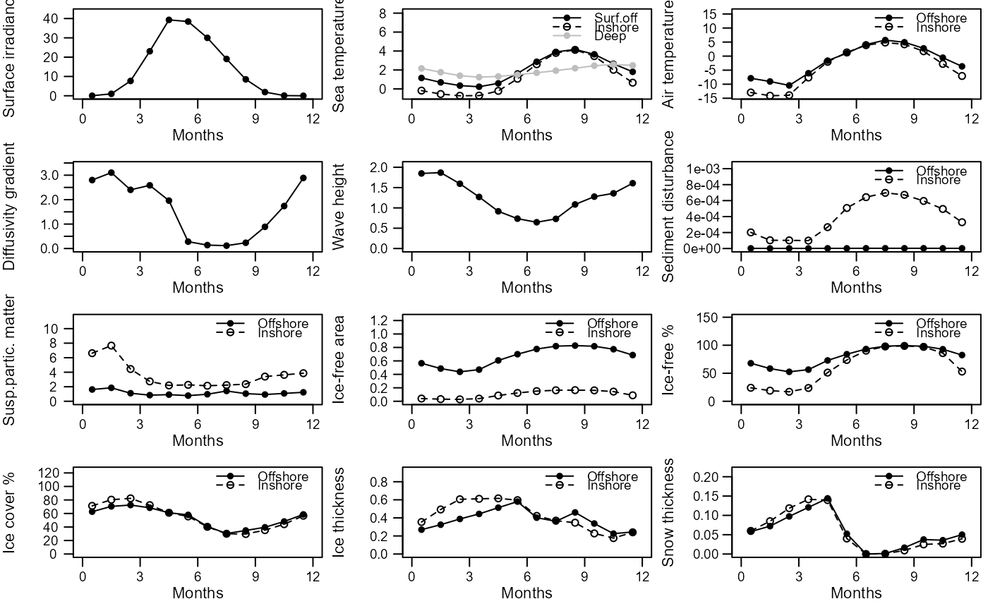
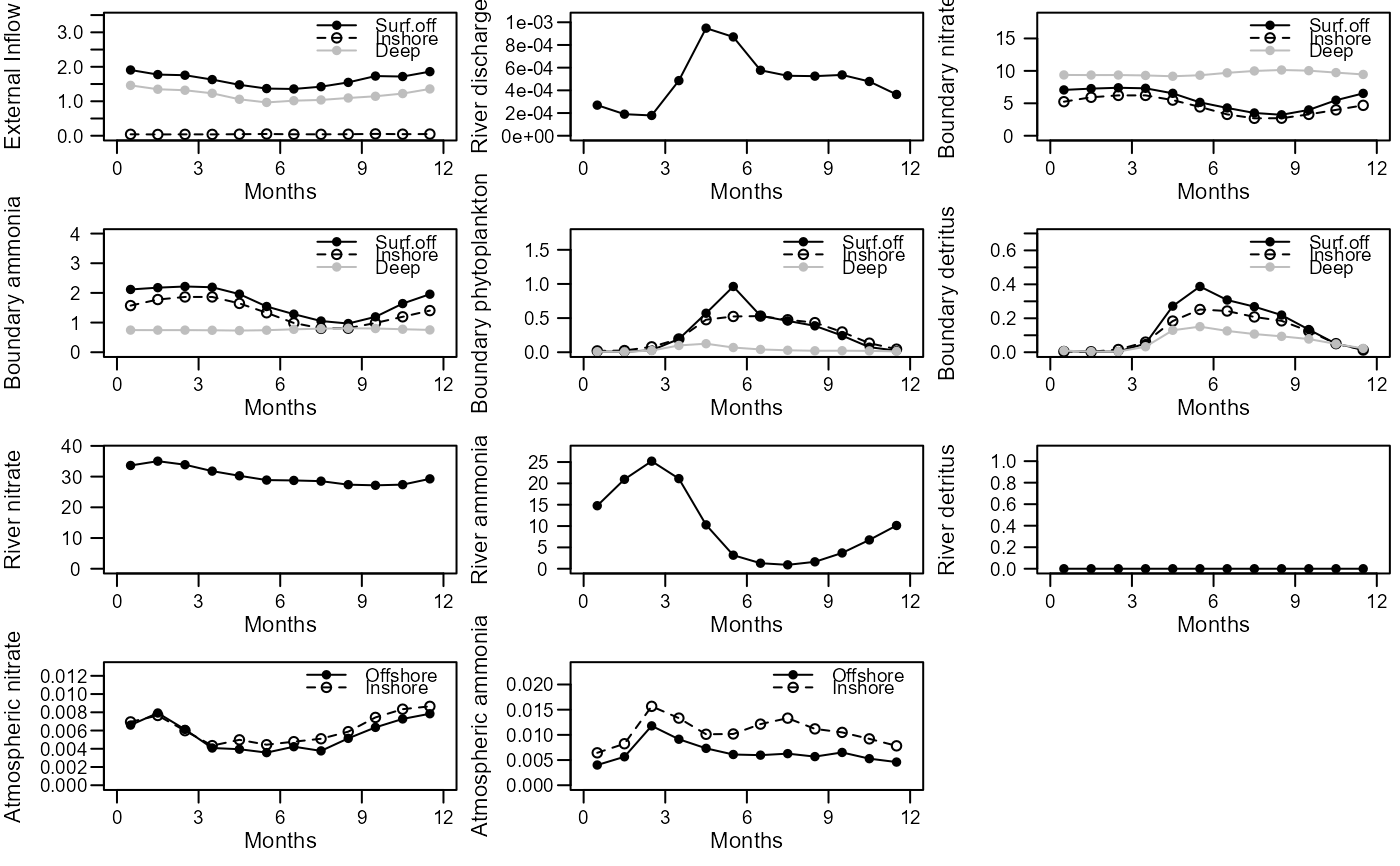
The function plots a multi-panel page of time series plots of monthly values of the environmental driving data for the model.
Units for the plotted variables are as follows:
Internal drivers (i.e. properties applied within the model domain)
Sea surface irradiance: uE/m2/d
Sea temperature: deg-C
Air temperature: deg-C
Vertical diffusivity gradient: m/d (derived from the vertical diffusivity (m2/s) and mixing length scale (m))
Inshore significant wave height: m
Proportion of seabed disturbed: /d (aggregated over the three sediment classes in each zone)
Suspended particulate matter: g/m3
Ice-free area: proportion of whole model domain (i.e. ice cover * zonal area)
Ice-free
Ice cover
Ice thickness: m
Snow thickness: m
Boundary drivers (i.e. properties applied at the boundaries of the model domain)
External inflows: m3 per m2 sea surface of model domain (derived from proportion input per layer volume, layer thicknesses and areas)
River discharge: m3 per m2 sea surface of model domain (derived from proportion input to inshore volume, and inshore layer thickness and area)
External boundary nitrate concentration: mMN/m3
External boundary ammonia concentration: mMN/m3
External boundary phytoplankton concentration: mMN/m3
External boundary detritus concentration: mMN/m3
River nitrate concentration: mMN/m3
River ammonia concentration: mMN/m3
River labile detritus concentration: mMN/m3
Atmospheric nitrate deposition flux: mMN/m2/d
Atmospheric ammonia deposition flux: mMN/m2/d
Examples
# Load the 2011-2019 version of the Barents Sea model supplied with the package:
model <- e2ep_read("Barents_Sea", "2011-2019")
#> Current working directory is...
#> 'C:/Users/jackl/OneDrive - University of Strathclyde/Documents/StrathE2E/strath-e-2-e-polar-webdev/docs/reference'
#> No 'results.path' specified so any csv data requested
#> will be directed to/from the temporary directory...
#> 'C:\Users\jackl\AppData\Local\Temp\RtmpSgdWsc'
#>
#> Model setup and parameters gathered from ...
#> StrathE2E2 package folder
#> Model results will be directed to/from ...
#> 'C:\Users\jackl\AppData\Local\Temp\RtmpSgdWsc/Barents_Sea/2011-2019/'
# Plot the annual cyles of internal driving data
e2ep_plot_edrivers(model,selection="INTERNAL")
 # Plot the annual cyles of boundary driving data
e2ep_plot_edrivers(model,selection="BOUNDARY")
# Plot the annual cyles of boundary driving data
e2ep_plot_edrivers(model,selection="BOUNDARY")
 # Direct the graphics output to a pdf file ...
# or jpeg("plot.jpg"), png("plot.png")
pdf(file.path(tempdir(), "plot.pdf"),width=8,height=6)
e2ep_plot_edrivers(model)
dev.off()
#> agg_png
#> 2
# Direct the graphics output to a pdf file ...
# or jpeg("plot.jpg"), png("plot.png")
pdf(file.path(tempdir(), "plot.pdf"),width=8,height=6)
e2ep_plot_edrivers(model)
dev.off()
#> agg_png
#> 2