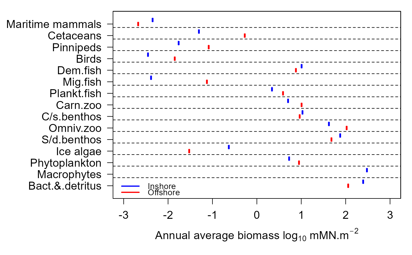
Plot showing the annual annual average biomass densities of each guild in the inshore and offshore zones, optionally with credible intervals.

Generate plots showing the annual average biomass densities of each guild in the ecology model in the inshore and offshore zones during the final year of a run. The default is to plot data from a single model run but if available, credible intervals of model output from a Monte Carlo analysis can also be plotted.

Usage

e2ep_plot_biomass(
  model,
  ci.data = FALSE,
  use.saved = FALSE,
  use.example = FALSE,
  results = NULL
)

Arguments

model: R-list object defining the model configuration used to generate the data and compiled by the e2ep_read() function.
ci.data: Logical. If TRUE plot credible intervals around model results based on Monte Carlo simulation with the e2ep_run_mc() function (default=FALSE).
use.saved: Logical. If TRUE use data from a prior user-defined run held as csv files data in the current results folder (default=FALSE).
use.example: NOT YET ENABLED. In future versions - Logical. If TRUE use pre-computed example data from the internal Barents Sea model rather than user-generated data (default=FALSE).
results: R-list object of baseline model output generated by the e2ep_run() function. Only needed if ci.data=FALSE, use.saved=FALSE and use.example=FALSE. (Default=NULL).

Value

graphical display in a new graphics window.

Details

Note that in this plot the biomass are expressed as mMN/m2, meaning that the mass in each zone has been scaled to the zonal sea surface area. So the data in this plot are area densities and not mass.

Arguments determine the source of model data to be plotted. These can be outputs from a single model run with data held in memory as a list object or in a saved csv file, or from a Monte Carlo simulation (using the function e2ep_run_mc()) to estimate credible intervals of model outputs. Generation of credible interval data is a long computing task, so example data for the Barents Sea model provided with the package are available as example data sets.

If credible intervals are plotted these are displayed as box-and-whiskers. The box spans 50 by a tick mark.

Examples

# Load the 2011-2019 version of the Barents Sea model supplied with the package, 
# run, and generate a plot:
    model <- e2ep_read("Barents_Sea", "2011-2019")
#> Current working directory is... 
#> 'C:/Users/jackl/OneDrive - University of Strathclyde/Documents/StrathE2E/strath-e-2-e-polar-webdev/docs/reference'
#> No 'results.path' specified so any csv data requested
#> will be directed to/from the temporary directory...
#> 'C:\Users\jackl\AppData\Local\Temp\RtmpSgdWsc'
#> 
#> Model setup and parameters gathered from ...
#> StrathE2E2 package folder
#> Model results will be directed to/from ...
#> 'C:\Users\jackl\AppData\Local\Temp\RtmpSgdWsc/Barents_Sea/2011-2019/'
    results <- e2ep_run(model, nyears=2)
    e2ep_plot_biomass(model, results=results)


# Direct the graphics output to a pdf file ... 
# or jpeg("plot.jpg"), png("plot.png")
    pdf(file.path(tempdir(), "plot.pdf"),width=4,height=6)
    e2ep_plot_biomass(model, results=results)
    dev.off()
#> agg_png 
#>       5 

# \donttest{
# Alternatively, plot the same data from a csv file saved by the e2ep_run() function. Here the
# csv output is directed to a temporary folder since results.path is not set in the e2ep_read()
# function call:
    results <- e2ep_run(model, nyears=2,csv.output=TRUE)
    dev.new()
    e2ep_plot_biomass(model, use.saved=TRUE)
#> Reading data from 'C:\Users\jackl\AppData\Local\Temp\RtmpSgdWsc/Barents_Sea/2011-2019/OFFSHORE_model_anav_biomass-base.csv'
#> Reading data from 'C:\Users\jackl\AppData\Local\Temp\RtmpSgdWsc/Barents_Sea/2011-2019/INSHORE_model_anav_biomass-base.csv'
# }

# For the same model, plot the example data with credible intervals:
# This example requires the StrathE2EPolarexamples supplementary data package.
if(require(StrathE2EPolarexamples)){
    e2ep_plot_biomass(model, ci.data=TRUE, use.example=TRUE)
}
#> Loading required package: StrathE2EPolarexamples
#> Warning: there is no package called 'StrathE2EPolarexamples'