Plot daily data on ecological outputs from the model over the final year of a run, optionally with credible intervals.

Generate a multi-panel set of one-year time series plots of selected outputs on the concentrations of state variables in the ecology model. The default is to plot data from a single model run but if available, credible intervals of model output from a Monte Carlo analysis can be plotted instead.

Usage

e2ep_plot_eco(
  model,
  selection = "NUT_PHYT",
  ci.data = FALSE,
  use.saved = FALSE,
  use.example = FALSE,
  results = NULL
)

Arguments

model: R-list object defining the baseline model configuration used to generate the data and compiled by the e2ep_read() function.
selection: Text string from a list identifying the group of model output variables to be plotted. Select from: "NUT_PHYT", "SEDIMENT", "ZOOPLANKTON", "FISH", "BENTHOS", "PREDATORS", "CORP_DISC", "MACROPHYTE", Remember to include the phrase within "" quotes.
ci.data: Logical. If TRUE plot credible intervals around model results based on Monte Carlo simulation with the e2ep_run_mc() function (default=FALSE).
use.saved: Logical. If TRUE use data from a prior user-defined run held as csv files data in the current results folder (default=FALSE).
use.example: NOT YET ENABLED. In future versions - Logical. If TRUE use pre-computed example data from the internal Barents Sea model rather than user-generated data (default=FALSE).
results: R-list object of model output generated by the e2ep_run() function. Only needed if ci.data=FALSE, use.saved=FALSE and use.example=FALSE. (Default=NULL).

Value

Graphical display in a new graphics window.

Details

Arguments determine the source of model data to be plotted. These can be outputs from a single model run with data held in memory as a list object or in a saved csv file, or from a Monte Carlo simulation (using the function e2ep_run_mc()) to estimate credible intervals of model outputs. Generation of credible interval data is a long computing task, so example data for the Barents Sea model provided with the package are available as an illustration.

If plotting of credible intervals is selected, results from the maximum likelihood model are shown by a red line. The median of the credible values distribution is shown my a solid black line. A grey-shaded area indicates the 50 of simulated values). Black dashed lines span the 99

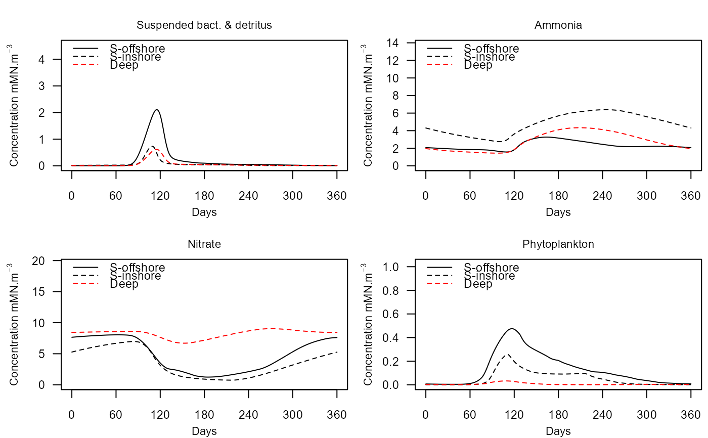
Variables to be plotted (and units) depending on values of "selection":

NUT_PHYT : Water column nitrate, ammonia, detritus and phytoplankton (mMN/m3)
IN_ICE : In-snow/ice concentrations of nitrate, ammonia, detritus and algae (mMN/m3 or mMN/m2 of snow or ice)
ZONE_ICE : Zonal area densities of snow/ice nitrate, ammonia, detritus and algae (mMN/m2 of zone)
SEDIMENT : Sediment porewater nitrate and ammonia, detritus and corpses (mMN/m3 or gN/gDW)
ZOOPLANKTON : Omnivorous and carnivorous zooplankton (mMN/m2)
FISH : Planktivorous and demersal fish and fish larvae (mMN/m2)
BENTHOS : Susp/dep and carn/scav benthos and benthos larvae (mMN/m2)
PREDATORS : Birds, pinnipeds, cetaceans and migratory fish (mMN/m2)
CORP_DISC : Corpses and discards (mMN/m2)
MACROPHYTE : Macrphytes and macrophyte debris (mMN/m2)

To direct the graph output to a file rather than the screen, wrap the e2ep_plot_eco() function call in a graphical device call: Since the plot pages contain different numbers of panels the suggested width:height ratios are as follows:

NUT_PHYT .... 1.5 : 1
IN_ICE ...... 1.5 : 1
ZONE_ICE .... 1.5 : 1
SEDIMENT ... 0.67 : 1
ZOOPLANKTON ... 1 : 1
FISH .......... 2 : 1
BENTHOS ....... 2 : 1
PREDATORS ..... 2 : 1
CORP_DISC ..... 1 : 1
MACROPHYTE .... 2 : 1

Examples

# Load the 2011-2019 version of the Barents Sea model supplied with the package, run, and
# generate a plot:
    model <- e2ep_read("Barents_Sea", "2011-2019")
#> Current working directory is... 
#> 'C:/Users/jackl/OneDrive - University of Strathclyde/Documents/StrathE2E/strath-e-2-e-polar-webdev/docs/reference'
#> No 'results.path' specified so any csv data requested
#> will be directed to/from the temporary directory...
#> 'C:\Users\jackl\AppData\Local\Temp\RtmpSgdWsc'
#> 
#> Model setup and parameters gathered from ...
#> StrathE2E2 package folder
#> Model results will be directed to/from ...
#> 'C:\Users\jackl\AppData\Local\Temp\RtmpSgdWsc/Barents_Sea/2011-2019/'
    results <- e2ep_run(model, nyears=2,csv.output=FALSE)
    e2ep_plot_eco(model, selection="NUT_PHYT",results=results)

    dev.new()
    e2ep_plot_eco(model, selection="ZOOPLANKTON",results=results)

# Direct the graphics output to a pdf file ... 
# or jpeg("plot.jpg"), png("plot.png")
    pdf(file.path(tempdir(), "plot.pdf"),width=8,height=4)
    e2ep_plot_eco(model, selection="FISH",results=results)
    dev.off()
#> agg_png 
#>       2 

# Load the 2011-2019 version of the Barents Sea model supplied with the package and
# plot example credible interval data:
# This example requires the StrathE2EPolarexamples supplementary data package.
if(require(StrathE2EPolarexamples)){
    e2ep_plot_eco(model, selection="BENTHOS",ci.data=TRUE,use.example=TRUE)
}
#> Loading required package: StrathE2EPolarexamples
#> Warning: there is no package called 'StrathE2EPolarexamples'