Chapter 9 Brief tour of optimization, sensitivity analysis and MCMC functions
See the package website for full details of parameter optimization, sensitivity and Monte Carlo methodology
9.1 Parameter optimization
Parameter optimization is a key part of developing a model implementation and assessing its credibility. The package includes a simulated annealing scheme for maximizing the likelihood of a set of empirical data on the state of the ecosystem given proposed parameters:
- e2e_optimize_eco() - Maximize the likelihood of observed ecosystem data by optimizing ecology model parameters
- e2e_optimize_hr() - Maximize the likelihood of observed ecosystem data by optimizing harvest ratio scaling parameters
- e2e_optimize_act() - Maximize the likelihood of observed ecosystem data or known harvest ratios by optimizing fishing activity parameters
The help pages for these functions provide a full explanation of the control options and example code for running them.
For the e2e_optimize_eco() process, details of the empirical target data to which the parameters are optimized is held in the model results object at resultsobject$final.year.outputs$annual.target.data, (where “resultsobject” is the name assigned to a given results object).
The correspondence between a given model results output and the target data is visualised by:
# Load the 1970-1999 version of the North Sea model supplied with the package, run, and
# generate a plot. Note that these are the observational data that were used as the target
# for optimizing the model parameters
model <- e2e_read("North_Sea", "1970-1999",silent=TRUE)
results <- e2e_run(model, nyears=3)
e2e_compare_obs(selection="ANNUAL", model, results=results)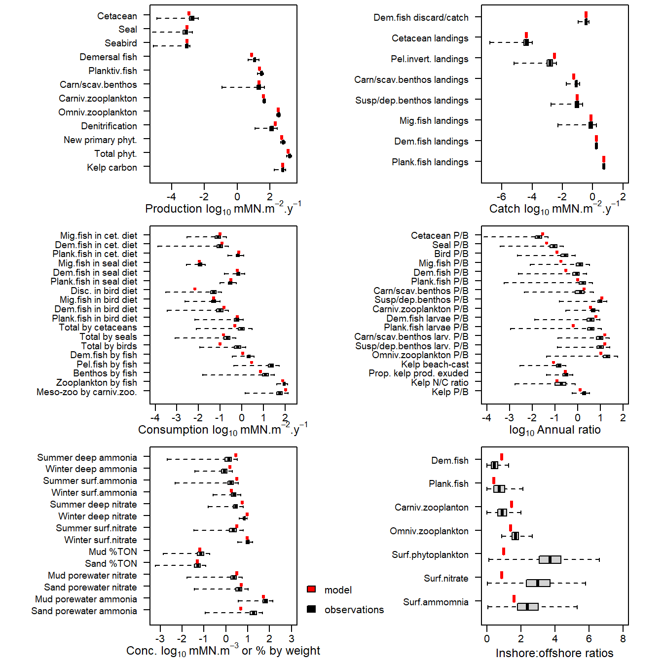
Figure 16. Comparison of 1970-1999 observational data from the North Sea (black box-plots) with corresponding values derived from a single run of the model (red symbols). For the observations, the box spans 50% of the distribution of observations and the whiskers 99%. The median is shown by a black tick mark.
9.2 Sensitivity analysis
Sensitivity analysis helps to highlight parameters which are:
- the most influence in the simulated annealing optimization process
- the most sensitive for any particular guild or process in the model
The e2e_run_sens() function performs a global analysis of parameter sensitivity using the Morris Method (Morris, 1991). This involves a factorial sampling scheme to generate parameter values for replicate model runs and generate values for the ‘Elementary Effect’ (EE) of each parameter. The mean and standard deviation of EE values over many runs allows ranking of the parameters in terms of the sensitivity of their effects on the model, and the strength of interactions with other parameters. For a review of global sensitivity analysis methods, including the Morris Method, see Wu et al. (2013).
- Morris, M.D. (1991). Factorial sampling plans for preliminary computational experiments. Technometrics, 33, 161-174.
- Wu, J., Dhingra, R., Gambhir, M. & Remais, J.V. (2013). Sensitivity analysis of infectious disease models: methods, advances and their application. Journal of the Royal Society Interface, 10: 20121018, 14pp.
The sensitivity analysis involves many thousands of model runs taking several days on a single processor. Procedures for parallel processing of are included in the package. Results for the North Sea model are included in the examples data package.
Sensitivity analysis results are visualized with the function e2e_plot_sens_mc()
# Plot the results of a parameter sensitivity analysis from the examples data package.
model<-e2e_read("North_Sea","1970-1999",silent=TRUE)
e2e_plot_sens_mc(model, selection="SENS", use.example=TRUE)
Reading example results from StrathE2E2examples data package for the North_Sea 1970-1999 model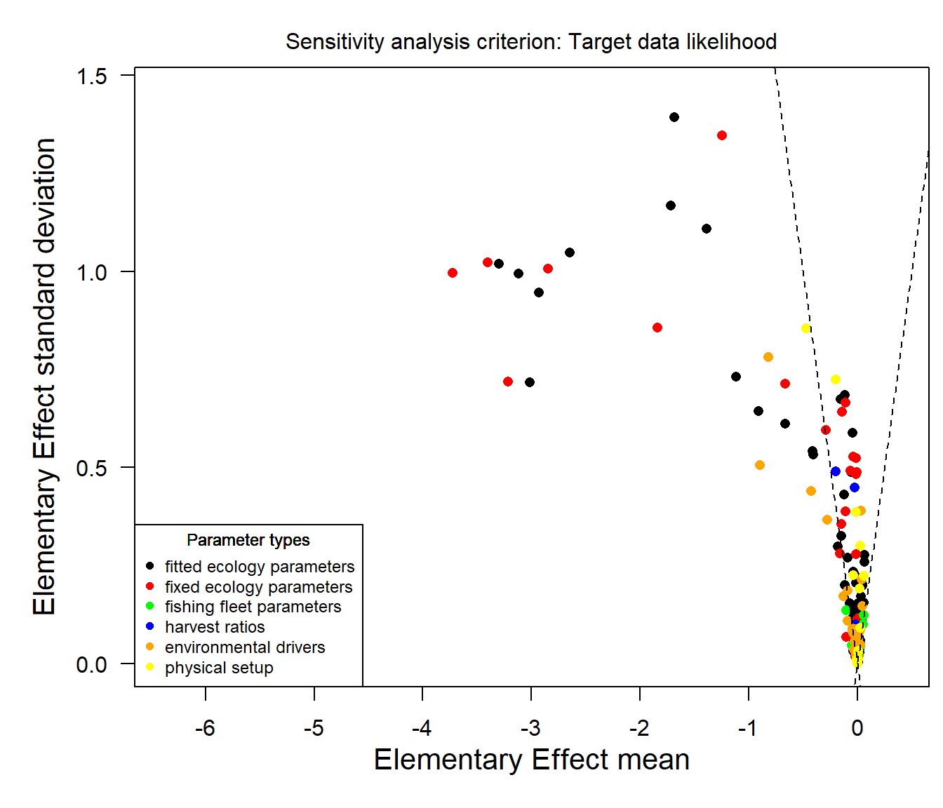
Figure 17. Sensitivity of the likelihood of observed data to each of the parameters for the 1970-1999 North Sea model from the examples data package. Each symbol in the plot represents a single parameter in the model. The x-axis represents the sensitivity of the overall likelihood of the observed data to each parameter. The y-axis represents the extent to which each parameter interacts with others. The parameters are colour-coded to indicate 6 different types - fitted and parameters of the ecology model, fishing fleet model parameters, fishery harvest ratios, environmental drivers, and physical configuration parameters. The wedge formed by the two dashed lines corresponds to \(\pm\) 2 standard errors of the mean, so for points falling outside of the wedge there is a significant expectation that the distribution of elementary effects is non-zero. For points falling within the wedge the distribution of elementary effects is not significantly different from zero.
You can examine the list of individual model parameters from the example dataset in descending order of Elementary Effect using:
head(StrathE2E2examples::example.results$North_Sea$variant_1970.1999$sorted_parameter_elementary_effects[,c(5,6,7,9,10,11)])
9.3 Monte Carlo analysis
The Monte Carlo scheme provided with the StrathE2E2 package (e2e_run_mc()) generates an ensemble of model runs by sampling the ecology model parameters from uniform distibutions centred on an initial (baseline) parameter set. Ideally, this should be the maximum likelihood parameter set arrived at by prior application the various optimization functions in the package to ‘fit’ the model to a suite of observational data on the state of ecosystem. Each iteration in the Monte Carlo scheme then generates a unique time series of model outputs at daily intervals, together with the overall likelihood of the obervational target data. From these data, the function then derives credible intervals of each output by weighting the values from each parameter set by the associated likelihood.
Running a Monte Carlo analysis is time consuming so the examples data package contains results for the North Sea model. Most of the results visualization functions that we explored earlier can also plot credible intervals of model output from these MC outputs. A few of examples are shown here:
# Compare credible intervals of model data derived from a Monte Carlo
# analysis with the observed target data:
model <- e2e_read("North_Sea", "1970-1999",silent=TRUE)
e2e_compare_obs(model, selection="ANNUAL",ci.data=TRUE,use.example=TRUE)
Reading example results from StrathE2E2examples data package for the North_Sea 1970-1999 model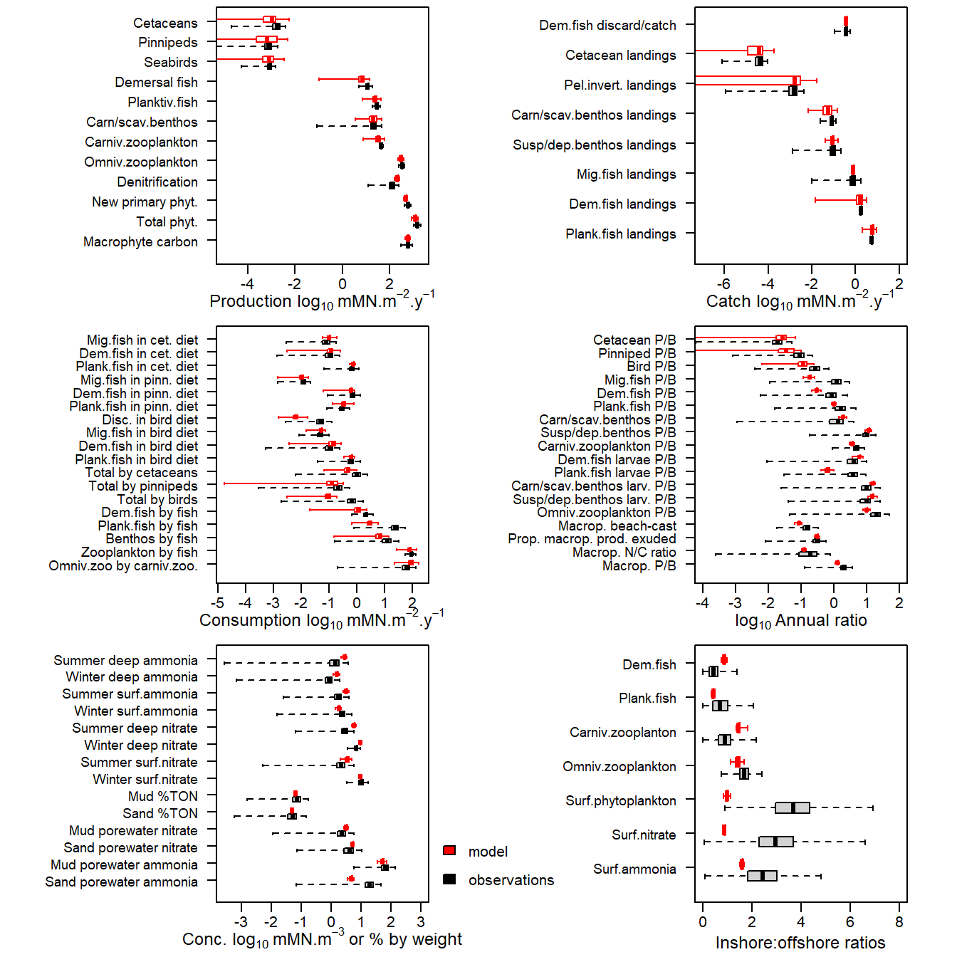
Figure 18. Comparison of 1970-1999 observational data from the North Sea (black box-plots) with credible intervals of corresponding values derived from a Monte Carlo analysis of the model (red box-plots). For both observations and model outputs, the box spans 50% of the distribution of observations and the whiskers 99%. The median is shown by a tick mark.
# Plot credible intervals of annual trophic indices derived from a Monte Carlo
# analysis for the 1970-1999 North Sea model:
model <- e2e_read("North_Sea", "1970-1999",silent=TRUE)
e2e_plot_trophic(model,ci.data=TRUE,use.example=TRUE)
Reading example results from StrathE2E2examples data package for the North_Sea 1970-1999 model
Warning in xtfrm.data.frame(x): cannot xtfrm data frames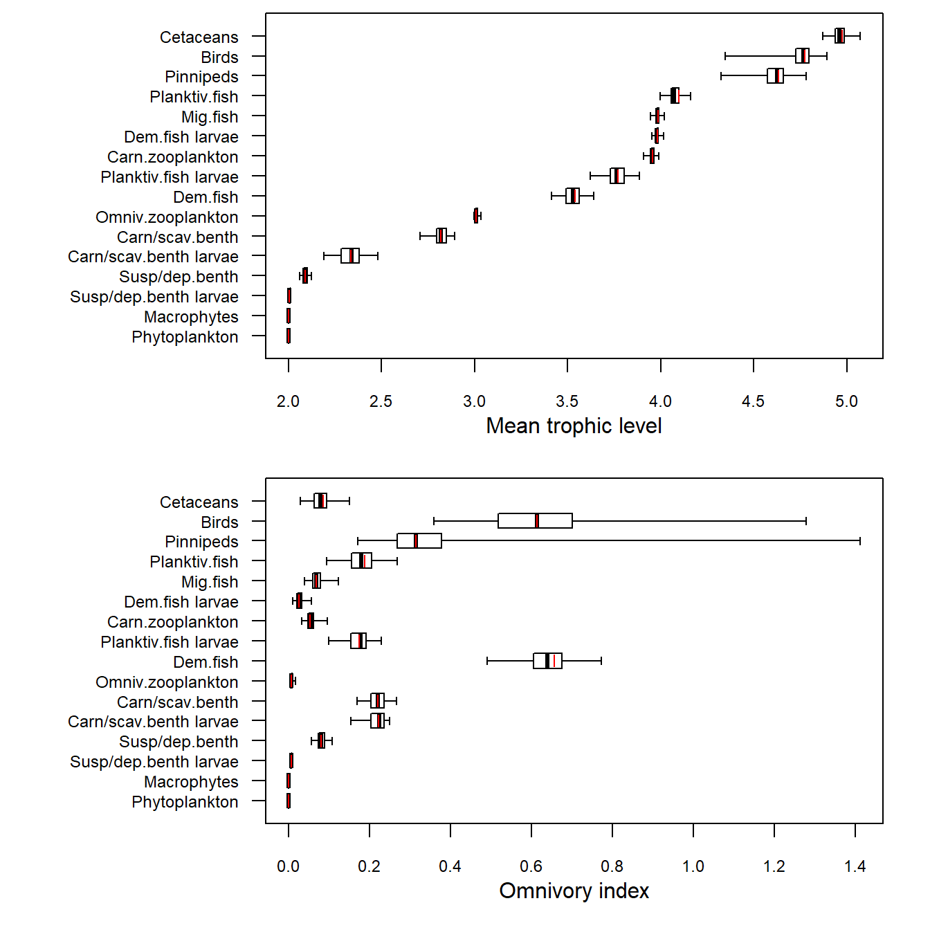
Figure 19. Credible intervals of annual mean trophic level and omnivory indices for the final year the 1970-1999 North Sea model. The box spans 50% of the distribution of credible outputs and the whiskers 99%. The median is shown by a black tick mark. The maximum likelihood value is indicated by a red tick mark.
# Plot credible intervals around the annual cycle of nutreint and phytoplankton
# outputs for the 1970-1999 North Sea model:
model <- e2e_read("North_Sea", "1970-1999",silent=TRUE)
e2e_plot_eco(model, selection="NUT_PHYT",ci.data=TRUE,use.example=TRUE)
Reading example results from StrathE2E2examples data package for the North_Sea 1970-1999 model
PlotOffshore zone upper layerandSuspended bact & detritus
PlotOffshore zone upper layerandAmmonia
PlotOffshore zone upper layerandNitrate
PlotOffshore zone upper layerandPhytoplankton
PlotOffshore zone lower layerandSuspended bact & detritus
PlotOffshore zone lower layerandAmmonia
PlotOffshore zone lower layerandNitrate
PlotOffshore zone lower layerandPhytoplankton
PlotInshore zoneandSuspended bact & detritus
PlotInshore zoneand Ammonia
PlotInshore zoneandNitrate
PlotInshore zoneandPhytoplankton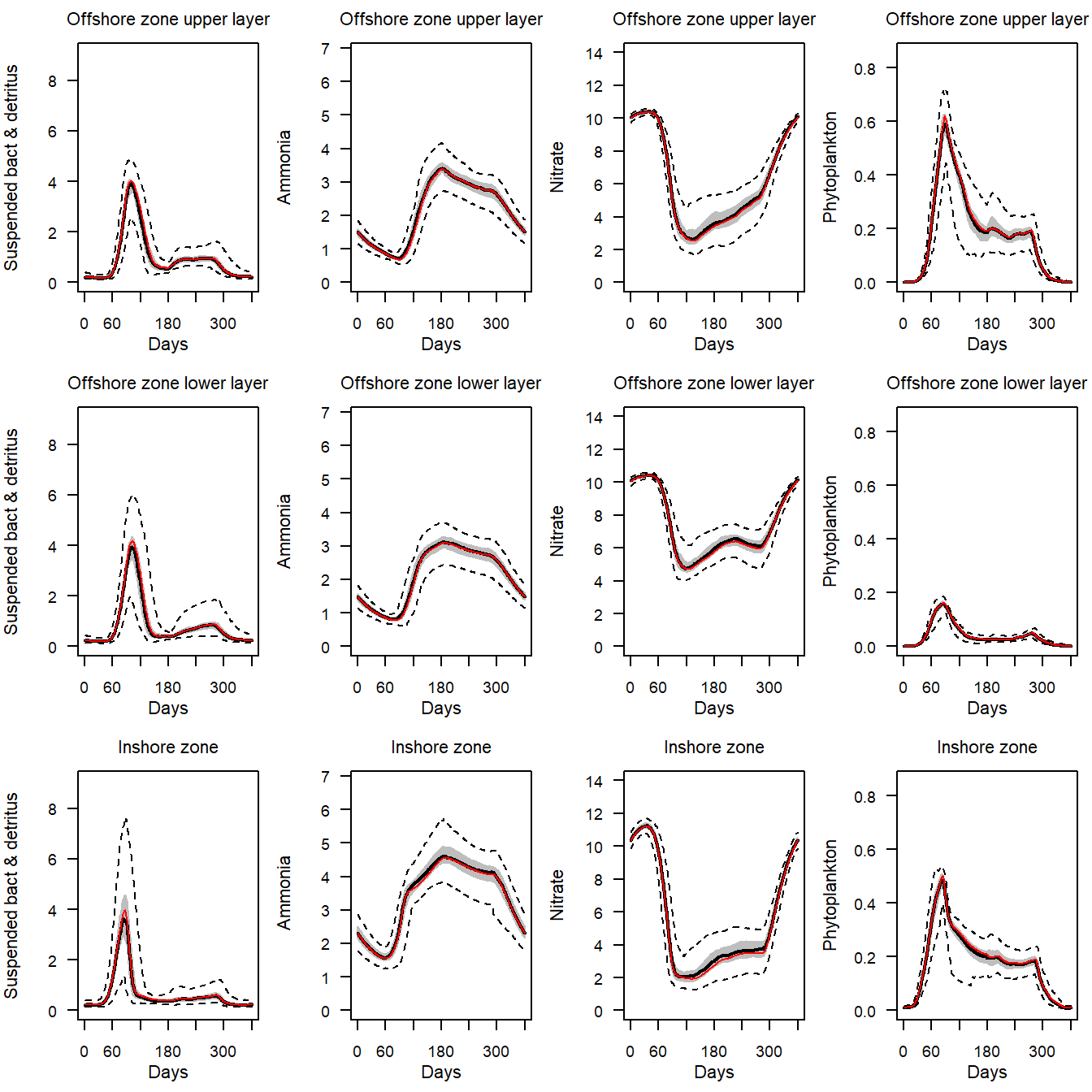
Figure 20. Credible intervals of daily interval nutrient, detritus and phytoplankton outputs for the final year the 1970-1999 North Sea model. The grey shading spans 50% of the distribution of credible outputs and the dashed lines 99%. The median is shown by a black line. The maximum likelihood value is indicated by a red line.
The full list of functions able to display either single run or credible intervals of model outputs is:
- e2e_compare_obs()
- e2e_compare_runs_box()
- e2e_plot_eco()
- e2e_plot_migration()
- e2e_plot_trophic()
- e2e_plot_biomass()