Chapter 6 More detailed visualization of model outputs
For the final year of a model run we can generate more detailed visualizations of the model results using the functions:
- e2e_plot_eco() - Plot annual cycles of ecological ouputs
- e2e_plot_catch() - Plot annual catches disaggregared by gear, guild, landings, discards
- e2e_plot_biomass() - Plot annual mean biomass of all guilds by inshore/offshore zone
- e2e_plot_migration() - Plot annual cycles of active migration rates between zones
- e2e_plot_trophic() - Plot annual mean trophic level and omnivory index of each guild
All of these functions have arguments to control the use of credible interval data from the examples package - which we will come to later. Here we just need the arguments to control plotting data from a single run.
6.1 Final year time series of ecological data (e2e_plot_eco())
Table 3. Relevant arguments of the functions e2e_plot_eco()
| Argument | Description |
|---|---|
| model | R-list object defining the model configuration compiled by the e2e_read() function |
| selection | Text string from a list identifying the group of model output variables to be plotted. Select from: “NUT_PHYT”, “SEDIMENT”, “ZOOPLANKTON”, “FISH”, “BENTHOS”, “PREDATORS”, “CORP_DISC”, “MACROPHYTE”, Remember to include the phrase within “” quotes |
| results | R-list object of model output generated by the e2e_run() function |
Table 4. Variables plotted (and units) given values of the argument “selection”
| selection | Variables plotted | Units |
|---|---|---|
| NUT_PHYT | Water column nitrate, ammonia, detritus and phytoplankton | mMN.m-3 |
| SEDIMENT | Sediment porewater nitrate and ammonia, detritus and corpses | mMN.m-3 or gN.gDW-1 |
| ZOOPLANKTON | Omnivorous and carnivorous zooplankton | mMN.m-2 |
| FISH | Planktivorous and demersal fish and fish larvae | mMN.m-2 |
| BENTHOS | Susp/dep and carn/scav benthos and benthos larvae | mMN.m-2 |
| PREDATORS | Birds, pinnipeds, cetaceans and migratory fish | mMN.m-2 |
| CORP_DISC | Corpses and discards | mMN.m-2 |
| MACROPHYTE | Macrphytes and macrophyte debris | mMN.m-2 |
Example plot of final year nutrient and phytoplankton time series
# Load the 1970-1999 version of the North Sea model supplied with the package,
# run, and generate a plot:
model <- e2e_read("North_Sea", "1970-1999",silent=TRUE)
results <- e2e_run(model, nyears=3)
e2e_plot_eco(model, selection="NUT_PHYT",results=results)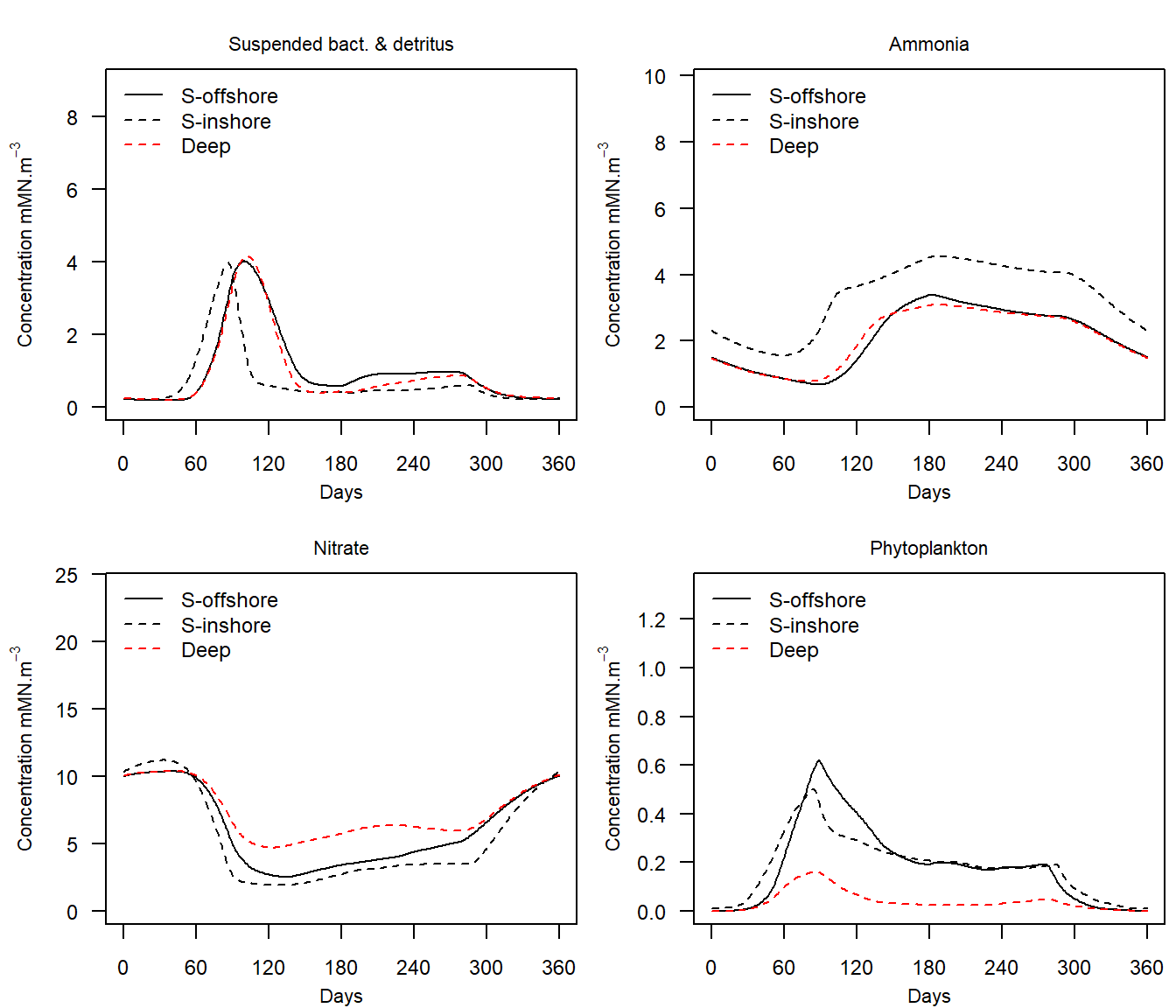
Figure 6. Annual cycles of nutrients and phytoplankton in the final year of a 1970-1999 North Sea model.
6.2 Plotting distributions of catches by gear and guild e2e_plot_catch()
Table 5. Arguments of the functions e2e_plot_catch()
| Argument | Description |
|---|---|
| model | R-list object defining the model configuration compiled by the e2e_read() function |
| results | List object of single-run model output generated by running the function e2e_run() function |
| selection | Text string from a list identifying the group of model output variables to be plotted. Select from: “BY_GUILD”, “BY_GEAR”. With the former, each panel represents a different guild; with the latter, each panel represnts a different gear. Remember to include the phrase within “” quotes |
Create stacked barplots of the distribution of offshore and inshore landings and discards across gears by guild, or across guilds by gears, in the final year of a model run.
Data in zonal landings and discards by guild and gear in the final year of a model run are generated as a standard output from the model, and saved both as csv files and in the results object returned by the e2e_run() function. This function organises these data in two different ways to display as barplots.
The first display is a multi-panel plot in which each panel represents a different guild, and the bars show the zonal landings by each gear. The alternative display has each panel as a different gear, and the bars show the landings and discards of each guild.
The unit of the displayed data are mMN.y-1 from the model domain as a whole, which is taken as being 1 m2.
e2e_plot_catch(model, results, selection="BY_GEAR")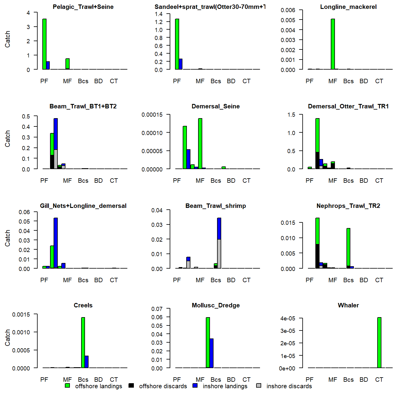
Figure 7. Annual landings and discards of each guild, by gear, in the final year of a run of the 1970-1999 North Sea model.
e2e_plot_catch(model, results, selection="BY_GUILD")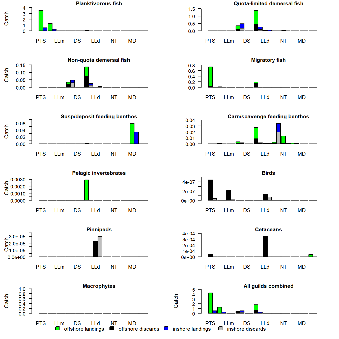
Figure 8. Annual landings and discards by each gear, by guild, in the final year of a run of the 1970-1999 North Sea model.
6.3 Zonal distributions of annual average biomass e2e_plot_biomass()
Table 6. Relevant arguments of the functions e2e_plot_biomass()
| Argument | Description |
|---|---|
| model | R-list object defining the model configuration compiled by the e2e_read() function |
| results | R-list object of model output generated by the e2e_run() function |
Generate plots showing the annual average biomass densities of each guild in the ecology model in the inshore (blue) and offshore (red) zones during the final year of a run.
Note that in this plot the biomass are expressed as mMN.m-2, meaning that the mass in each zone has been scaled to the zonal sea surface area. So the data in this plot are area densities and not mass.
e2e_plot_biomass(model, results=results)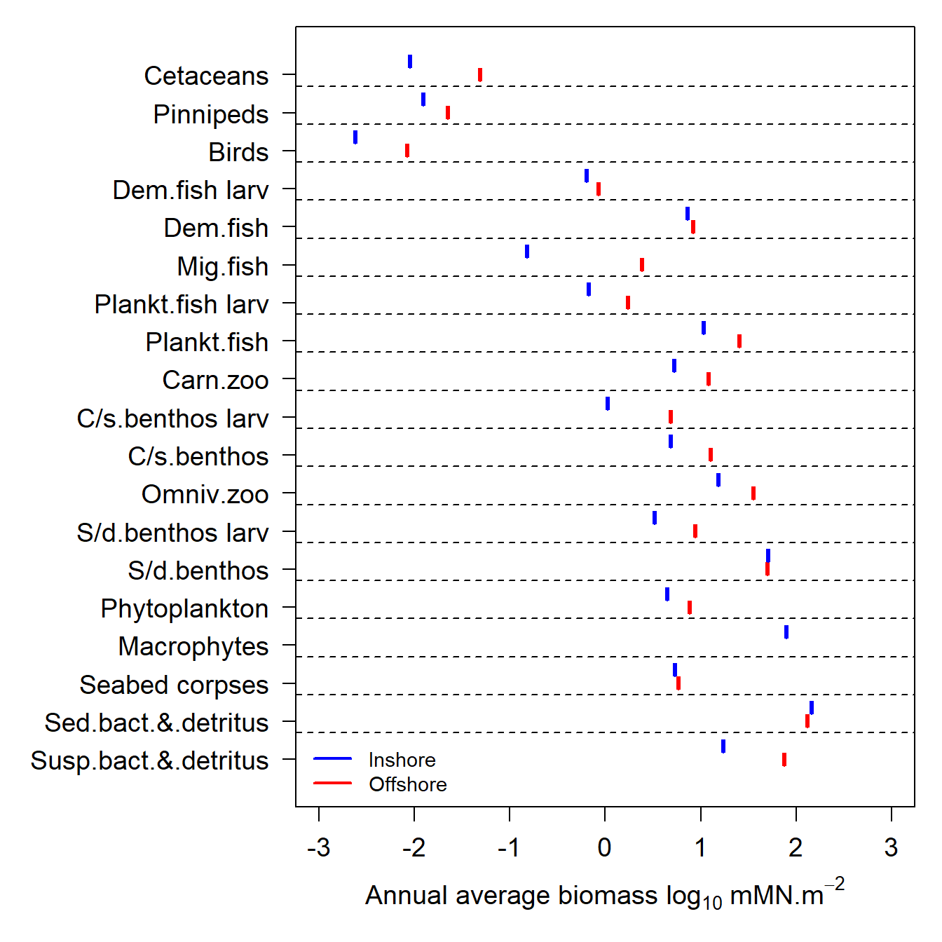
Figure 9. Annual average biomass densities for the final year of a single run of the 1970-1999 North Sea model.
6.4 Final year time series of migration fluxes (e2e_plot_migration())
Table 7. Relevant arguments of the functions e2e_plot_migration()
| Argument | Description |
|---|---|
| model | R-list object defining the model configuration compiled by the e2e_read() function |
| results | R-list object of model output generated by the e2e_run() function |
Each panel of the plot shows a time-series of the net flux densities (mMN.d-1 in the model domain as a whole, assumed to be 1 m2 sea surface area) of one of the migratory guilds in the model (all three guilds of fish, birds, pinnipeds and cetaceans) between the inshore and offshore zones of the model, over the final year of a run. These migration fluxes are the dynamic product of gradients in the ratio of food concentration to predator concentration across the inshore-offshore boundary. Positive values of the net migration flux indicate net movement from the offshore to inshore zone. Negative values indicate net movement from inshore to offshore.
e2e_plot_migration(model, results=results)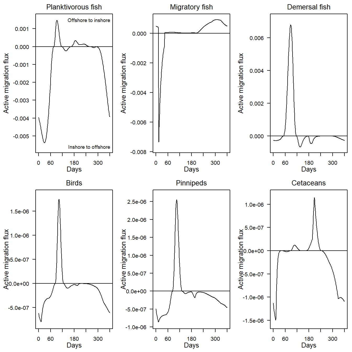
Figure 10. Annual cycles of migration fluxes between the offshore and inshore zones in the final year of a 1970-1999 North Sea model.
6.5 Plotting mean trophic level and omnivory indices e2e_plot_trophic()
Table 8. Relevant arguments of the functions e2e_plot_trophic()
| Argument | Description |
|---|---|
| model | R-list object defining the model configuration compiled by the e2e_read() function |
| results | R-list object of model output generated by the e2e_run() function |
Generate a two-panel plot showing: (upper panel) the mean trophic level of each guild in the ecology model, and (lower panel) the omnivory index of each guild. The data are generated by the NetIndices package from a flow matrix of nutrient fluxes through, into and out of the ecosystem during the final year of a run. The data are generated automatically as part of the output from every call of the e2e_run() function.
Note the the NetINdices package assigns trophic level 1 to inorganic nutrients and detritus, to autotrophs and detritivores are ranked as trophic level 2.
e2e_plot_trophic(model, results=results)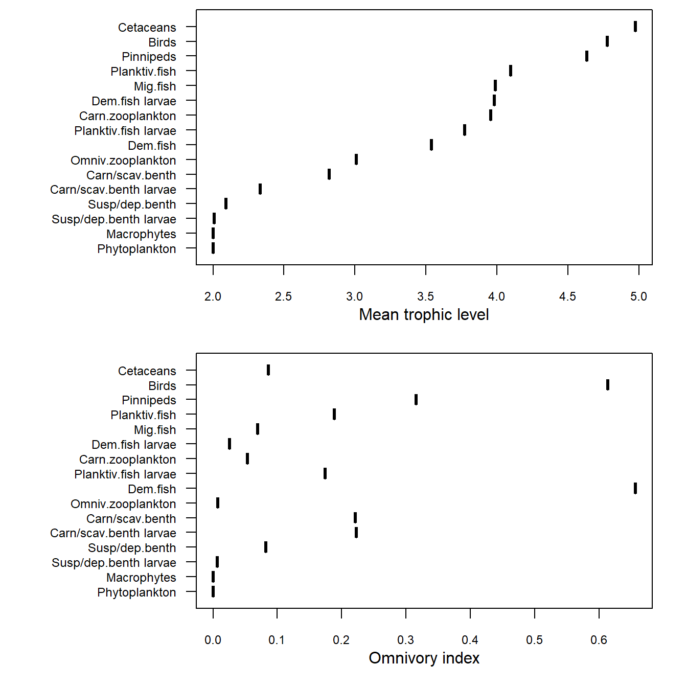
Figure 11. Annual mean trophic level and omnivory indices for the final year of a single run of the 1970-1999 North Sea model.