Chapter 4 Let’s get started
4.1 Loading the package
To start a session, begin by loading the package:
library(StrathE2E2)
To check the details of the package you have installed:
e2e_info_pk()
Package: StrathE2E2
Version: 4.0.0
Title: End-to-End Marine Food Web Model
Author: Michael Heath [aut], Ian Thurlbeck [ctb]
Maintainer: Michael Heath <m.heath@strath.ac.uk>
Depends: R (>= 3.6.0),
Imports: deSolve, methods, NetIndices
Description: A dynamic model of the big-picture, whole ecosystem
        effects of hydrodynamics, temperature, nutrients, and fishing
        on continental shelf marine food webs. The package is described
        in: Heath, M.R., Speirs, D.C., Thurlbeck, I. and Wilson, R.J.
        (2021) <doi:10.1111/2041-210X.13510> StrathE2E2: An R package
        for modelling the dynamics of marine food webs and fisheries.
        Methods in Ecology and Evolution 12, 280-287.
License: GPL (>= 2)
LazyData: yes
NeedsCompilation: yes
Date: 2022-10-07
URL: https://www.marineresourcemodelling.maths.strath.ac.uk/strathe2e/
Suggests: knitr, StrathE2E2examples, testthat (>= 2.1.0)
VignetteBuilder: knitr
Encoding: UTF-8
RoxygenNote: 7.1.1
Additional_repositories:
        https://www.marineresourcemodelling.maths.strath.ac.uk/strathe2e/articles/Pkg_versions.html
Packaged: 2022-10-11 00:31:14 UTC; ais04103
Built: R 4.1.2; x86_64-w64-mingw32; 2022-10-17 17:39:56 UTC; windows

-- File: C:/Users/jackl/Documents/R/win-library/4.1/StrathE2E2/Meta/package.rds
4.2 Load a model
The package has two variants of a model of the North Sea embedded within it:
e2e_ls()
Current working directory is 'C:/Users/jackl/OneDrive - University of Strathclyde/Documents/StrathE2E/training course/StrathE2E2/4.0.0'
List of package models in system folder "extdata/Models", with examples of how to read them:
 Model: "North_Sea"
  Variant: "1970-1999"  model <- e2e_read("North_Sea", "1970-1999")
  Variant: "2003-2013"  model <- e2e_read("North_Sea", "2003-2013")
You can view details of these models using the function e2e_info_md():
e2e_info_md()
Path to the model is: 'C:/Users/jackl/Documents/R/win-library/4.1/StrathE2E2/extdata/Models'
 [1] "Model region      : North_Sea"
 [2] "StrathE2E2 version: 4.0.0"
 [3] ""
 [4] "Model variant name: 1970-1999"
 [5] "Release date      : 30-05-2022"
 [6] "Implementation originally produced in the NERC Marine Ecosystem Programme (https://marine-ecosystems.org.uk/)"
 [7] "Driving data represent a climatological annual cycle for the period 1970-1999"
 [8] "Hydrodynamnic driving data from NEMO-ERSEM 7km model (https://www.uk-ssb.org/science_components/work_package_4/)"
 [9] "Nutrient driving data from ICES and BODC data archives and informed by NEMO-ERSEM"
[10] "Atmospheric driving data from EMEP (https://www.emep.int/)"
[11] "River driving data from a statistical models of rainfall river flow and nutrent monitoring data (https://strathprints.strath.ac.uk/18588/6/strathprints018588.pdf)"
[12] "Fishing data from ICES and STECF (https://www.ices.dk/data/dataset-collections/Pages/Fish-catch-and-stock-assessment.aspx and https://stecf.jrc.ec.europa.eu/dd/fdi)"
[13] "Setup parameters modified May 2022 to be consistent with StrathE2E 4.0.0"
[14] "Documentation: https://www.marineresourcemodelling.maths.strath.ac.uk/resources/StrathE2E2/documents/4.0.0/StrathE2E2_North_Sea_model.pdf"
[15] ""
[16] "Model variant name: 2003-2013"
[17] "Release date      : 30-05-2022"
[18] "Implementation originally produced in the NERC Marine Ecosystem Programme (https://marine-ecosystems.org.uk/)"
[19] "Driving data represent a climatological annual cycle for the period 2003-2013"
[20] "Hydrodynamnic driving data from NEMO-ERSEM 7km model (https://www.uk-ssb.org/science_components/work_package_4/)"
[21] "Nutrient driving data from ICES and BODC data archives and informed by NEMO-ERSEM"
[22] "Atmospheric driving data from EMEP (https://www.emep.int/)"
[23] "River driving data from a statistical models of rainfall river flow and nutrent monitoring data (https://strathprints.strath.ac.uk/18588/6/strathprints018588.pdf)"
[24] "Fishing data from ICES and STECF (https://www.ices.dk/data/dataset-collections/Pages/Fish-catch-and-stock-assessment.aspx and https://stecf.jrc.ec.europa.eu/dd/fdi)"
[25] "Setup parameters modified May 2022 to be consistent with StrathE2E 4.0.0"
[26] "Documentation: https://www.marineresourcemodelling.maths.strath.ac.uk/resources/StrathE2E2/documents/4.0.0/StrathE2E2_North_Sea_model.pdf"
[27] ""
Here is a map of the North Sea model domain:
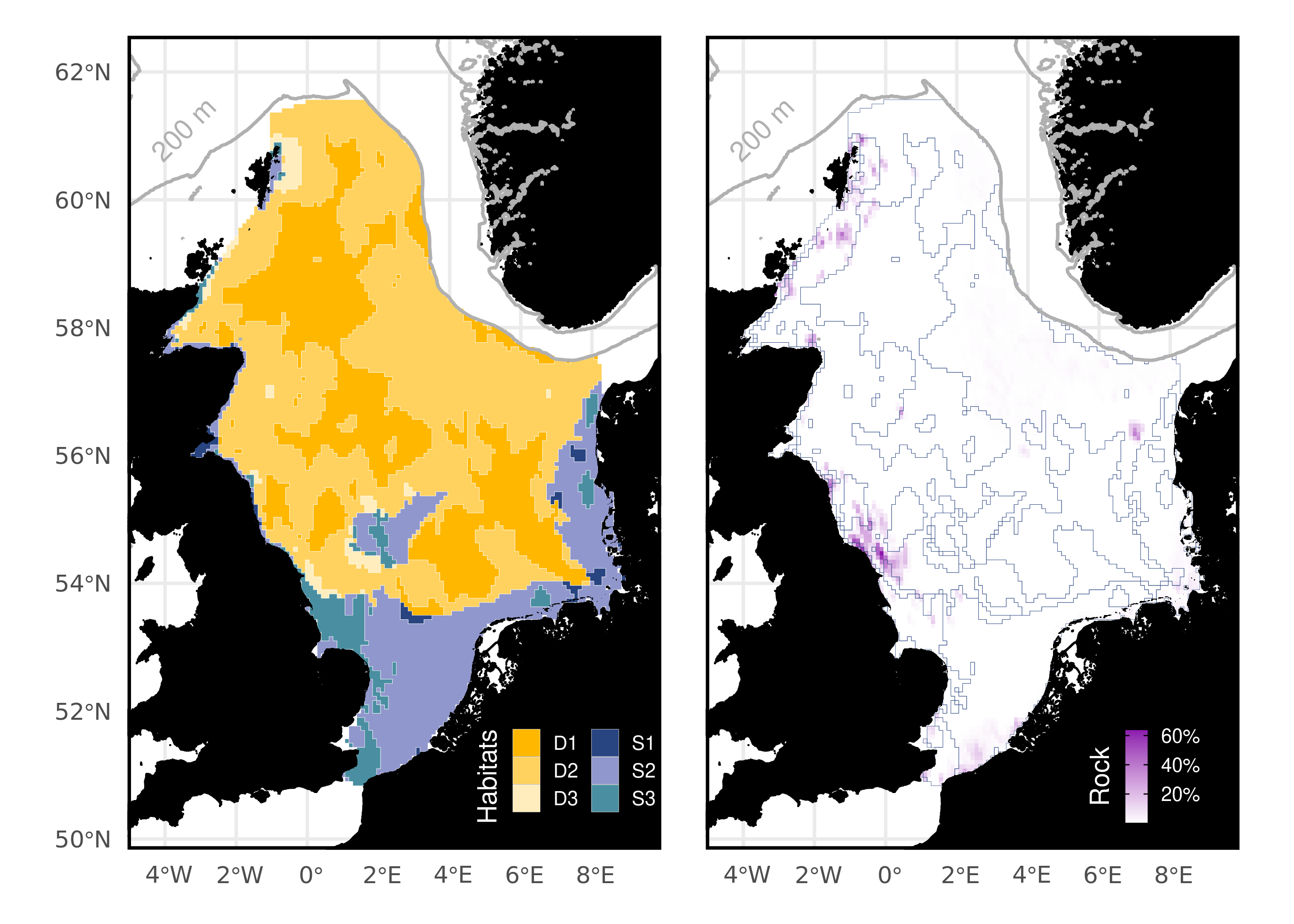
Figure 1. Domain of the North Sea model include in the package showing the seabed habiats in the inshore and offshore zones.
e2e_read() is a key function in the package which returns a list object containing all of the input data and parameters gathered from a set of csv files that define the model implementation.
To read the 1970-1999 North Sea model:
model <- e2e_read("North_Sea", "1970-1999")   # Read the 1970-1999 North Sea model from within the package
Current working directory is...
'C:/Users/jackl/OneDrive - University of Strathclyde/Documents/StrathE2E/training course/StrathE2E2/4.0.0'
No 'results.path' specified so any csv data requested
will be directed to/from the temporary directory...
'C:\Users\jackl\AppData\Local\Temp\RtmpqsmriQ'

Model setup and parameters gathered from ...
StrathE2E2 package folder
Model results will be directed to/from ...
'C:\Users\jackl\AppData\Local\Temp\RtmpqsmriQ/North_Sea/1970-1999/'
4.3 Viewing the model input data
You can view the climatological annual cycles of input environmental driving data in the model object using the function e2e_plot_edrivers(). This displays the following data:
Table 1. Environmental input data dispalayed in each panel of the plot produced by e2e_plot_edrivers()
| Data | Units | Comments |
|---|---|---|
| Sea surface irradiance | \(\mu\)E.m-2.d-1 | |
| Suspended particulate matter | g.m-3 | |
| Temperature | deg-C | |
| Vertical diffusivity gradient | m.d-1 | derived from the vertical diffusivity (m2.s-1) and mixing length scale (m) |
| External inflows | m3 per m2 sea surface of model domain | derived from proportion input per layer volume, layer thicknesses and areas |
| River discharge | m3 per m2 sea surface of model domain | derived from proportion input to inshore volume, and inshore layer thickness and area |
| Inshore significant wave height | m | |
| Proportion of seabed disturbed | d-1 | aggregated over the three sediment classes in each zone |
| External boundary nitrate concentration | mMN.m-3 | |
| External boundary ammonia concentration | mMN.m-3 | |
| External boundary phytoplankton concentration | mMN.m-3 | |
| External boundary detritus concentration | mMN.m-3 | |
| River nitrate concentration | mMN.m-3 | |
| River ammonia concentration | mMN.m-3 | |
| Atmospheric nitrate deposition flux | mMN.m-2.d-1 | area averaged flux density over each zone |
| Atmospheric ammonia deposition flux | mMN.m-2.d-1 | area averaged flux density over each zone |
e2e_plot_edrivers(model)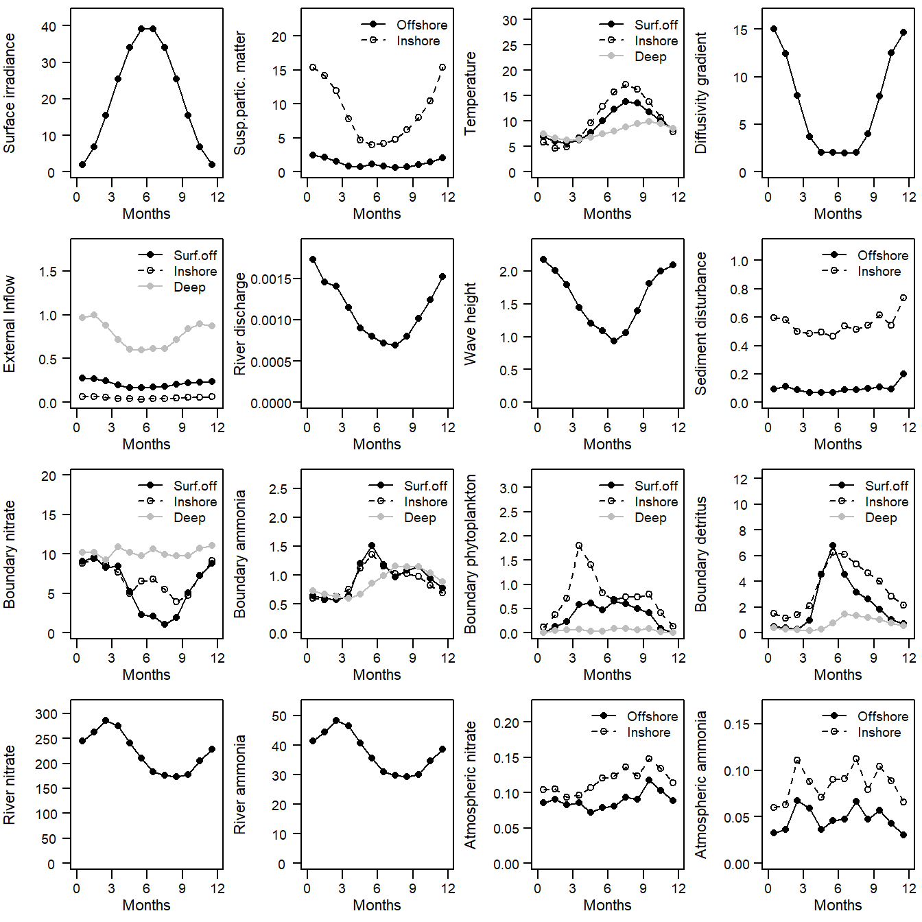
Figure 2. Plot of climatological annual cycles of the environmental drivers of the 1970-1999 North Sea model
The other main sets of input data to the model concerns the fishing fleets. The fishing fleet model can represent up to 12 different categories of fishing, each defined by its:
- activity rate
- proportional spatial distribution across the inshore and offshore zone and seabed habitats
- catching power for each of the catchable guilds in the model (i.e. selectivity)
- discard rate for each of the catchable guilds
- processing-at-sea rate for each of the catchable guilds (which generates offal)
- seabed abrasion rate
- proportionality coefficient relating effort (activity x power) to fishing mortality rate on each guild
The fishing fleet model integrates across the fleets and generates the overall harvest ratio (equivalent to fishing mortality rate), discard and offal production rates for each guild, and the seabed abrasion rates for each seabed habitat.
You can view the fishing fleet input data using the function e2e_plot_fdrivers(). This function has two arguments:
Table 2. Arguments of the functions e2e_plot_fdrivers()
| Argument | Description |
|---|---|
| model | R-list object defining a model configuration and compiled by the e2e_read() function |
| selection | Text string from a list identifying the class of fishing-related driving data to be plotted. Select from: “ACTIVITY”, “ABRASION”, “HARVESTR”, “DISCARDS”, “OFFAL”. Remember to include the phrase within “” quotes |
Regardless of the variable selected, the function returns both a graphical image and a list object containing the matix of data plotted and vectors of the axis labels, which uses can use to generate your own plots if desired.
Example use of e2e_plot_fdrivers() using the argument selection = “ACTIVITY”. This plots a matrix of seabed habitats vs fishing gears with each cell shaded to indicate \(log_e\) transformed activity density (white = 0, purple = high).
The spatial distribution of fishing gear activity in the model is defined by two input data sets: * Vector of whole domain activity density of each fishing gear (s.d-1 per m2 of whole model domain) * Matrix of the proportional distribution of whole domain activity density of each gear (rows) across seabed habitats (columns)
The activity density of each gear in each habitat is then obtained by multiplying the whole domain activity density into the proportional distribution matrix, and dividing by the area-proportions of habitats in the domain. The units of habitat-specific activity density are then (s.d-1.m-2).
# Load the 1970-1999 version of the North Sea model supplied with the package,
# run, and generate a plot:
plotted_data<-e2e_plot_fdrivers(model, selection="ACTIVITY")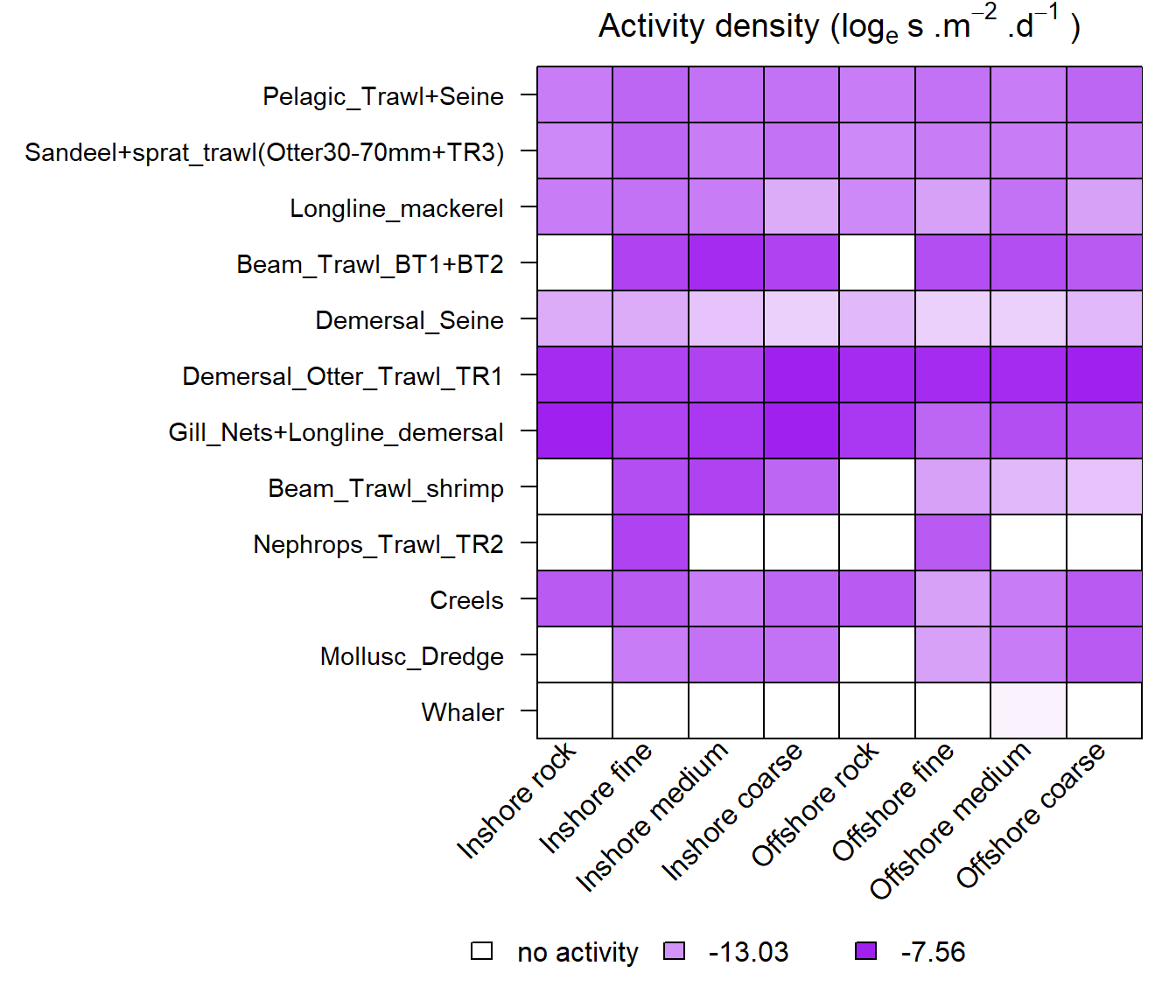
Figure 3. Distribution of gear activity rates across habitats in the 1970-1999 North Sea model.