Chapter 7 Writing code to create model scenarios
Typical use of the model might involve
comparing a baseline run with a scenario run involving some changes in driving data (e.g. different temperature conditions or different activity rates of selected gears),
conducting an analysis of the sensitivity to systematic changes in driving data (e.g. incrememts in river nutrient inputs over some range of values).
The most efficient way to create model scenarios is to write scripts to modify the R list object created by the e2e_read() function, assigning a unique identifier to the outputs from each run.
The scope for developing fishing and/or environmemtal scenarios by coding to modify a default model object is limitless, but requires an understanding of the structure and content of the list object produced by the e2e_read() function. Use the R str() function to explore the list and its sub-components, and consult the StrathE2E2 Technical Manual.
model<-e2e_read("North_Sea", "2003-2013",silent=TRUE)
str(model,max.level=1)                    # View the top 2 levels of input list object
List of 2
 $ setup:List of 7
 $ data :List of 9
str(model$data,max.level=1)                    # View the contents of the **data** level in the mopdel object
List of 9
 $ fixed.parameters   :List of 51
 $ fitted.parameters  :List of 171
 $ physical.parameters:List of 66
 $ physics.drivers    :'data.frame':    12 obs. of  28 variables:
 $ chemistry.drivers  :'data.frame':    12 obs. of  27 variables:
 $ biological.events  :'data.frame':    26 obs. of  2 variables:
 $ fleet.model        :List of 19
 $ initial.state      :List of 416
 $ biology.scenarios  :List of 2
To mine deeper into the model object, for example, to show the fleet model inputs:
str(model$data$fleet.model,max.level=1)
List of 19
 $ gear_labels                : chr [1:12] "Pelagic_Trawl+Seine" "Sandeel+sprat_trawl(Otter30-70mm+TR3)" "Longline_mackerel" "Beam_Trawl_BT1+BT2" ...
 $ gear_codes                 : chr [1:12] "PTS" "SST" "LLm" "BTf" ...
 $ gear_activity              : num [1:12] 2.17e-06 4.23e-06 1.68e-06 1.15e-05 1.72e-08 2.16e-05 7.92e-06 1.27e-05 1.72e-05 2.40e-05 ...
 $ gear_group_rel_power       :'data.frame':    12 obs. of  10 variables:
 $ gear_group_discard         :'data.frame':    12 obs. of  10 variables:
 $ gear_group_gutting         :'data.frame':    12 obs. of  10 variables:
 $ gear_ploughing_rate        : num [1:12] 0 8.8 0 54.1 22.4 17.1 0 13.5 78.9 0 ...
 $ gear_habitat_activity      :'data.frame':    12 obs. of  9 variables:
 $ HRscale_vector             : Named num [1:10] 0.0697 0.0755 0.3696 12.662 0.6301 ...
  ..- attr(*, "names")= chr [1:10] "PF_HR_scale" "DF_HR_scale" "MF_HR_scale" "SB_HR_scale" ...
 $ HRscale_vector_multiplier  : int [1:10] 1 1 1 1 1 1 1 1 1 1
 $ offal_prop_live_weight     : num 0.1
 $ gear_mult                  : int [1:12] 1 1 1 1 1 1 1 1 1 1 ...
 $ quota_nonquota_parms_vector: num [1:6] 0.16 0.07 0.67 0.02 0.4 0.02
 $ DFsize_SWITCH              : num 0
 $ DFdiscard_SWITCH           : num 1
 $ plough_thickness           : num 0.05
 $ plough_depth_vector        : num [1:9] 0 0.4316 0.0582 0.0455 0 ...
 $ BSmort_gear                : num 0.2
 $ BCmort_gear                : num 0.2
Below is an example of code to configure and run a scenario case of the the 2003-2013 North Sea model. It involves editing the fleet.model data to set the activity of demersal beam trawlers to zero.
The identities of the fishing fleets in the model are listed in:
model$data$fleet.model$gear_labels
 [1] "Pelagic_Trawl+Seine"
 [2] "Sandeel+sprat_trawl(Otter30-70mm+TR3)"
 [3] "Longline_mackerel"
 [4] "Beam_Trawl_BT1+BT2"
 [5] "Demersal_Seine"
 [6] "Demersal_Otter_Trawl_TR1"
 [7] "Gill_Nets+Longline_demersal"
 [8] "Beam_Trawl_shrimp"
 [9] "Nephrops_Trawl_TR2"
[10] "Creels"
[11] "Mollusc_Dredge"
[12] "Whaler"
The activity rates of each gear in the ‘out of the box’ model are listed in:
model$data$fleet.model$gear_activity
 [1] 2.17000e-06 4.23000e-06 1.68000e-06 1.15000e-05 1.72000e-08 2.16000e-05
 [7] 7.92000e-06 1.27000e-05 1.72000e-05 2.40000e-05 3.11000e-06 1.27413e-08
The vector gear_mult (length 12) is a set of multipliers which are applied to the ‘out of the box’ activity rates (defaults = 1):
model$data$fleet.model$gear_mult
 [1] 1 1 1 1 1 1 1 1 1 1 1 1
Code to build a model scenario
# Example of code to run a baseline case of the North Sea model with 2003-2013 conditions,
# and then edit the model list object to create a scenario run with beam trawl activity
# reset to zero
#--------------------------------------------------------
# Read the embedded North Sea 2003-2013 model and assign an identifier for the results
base_model<-e2e_read("North_Sea", "2003-2013",model.ident="base",silent=TRUE)
# Here model.ident assigns a text string to add to any output csv files
#
# Run the model for 3 years and save the results to a named list object
base_results<-e2e_run(base_model,nyears=3)
# You could visualize the output from the run but we know this shows a repeating annual cycle with no trend)
# e2e_plot_ts(base_model,base_results,"ECO")
# copy the baseline model list object to a new model list
scenario_model<-base_model
#
# Reset the activity multiplier of demersal beam trawlers to zero
# Beam trawlers are element 4 of the fleet list
scenario_model$data$fleet.model$gear_mult[4] <- 0
# Assign a new identifier for any .csv outputs
scenario_model$setup$model.ident <- "no_beam"
#
# Run the model for 10 years and save the results to a new list object
scenario_results<-e2e_run(scenario_model,nyears=10)
# Visualize the output from the run (should show trends in some outputs due to the change in gear activity)
e2e_plot_ts(scenario_model,scenario_results,"ECO")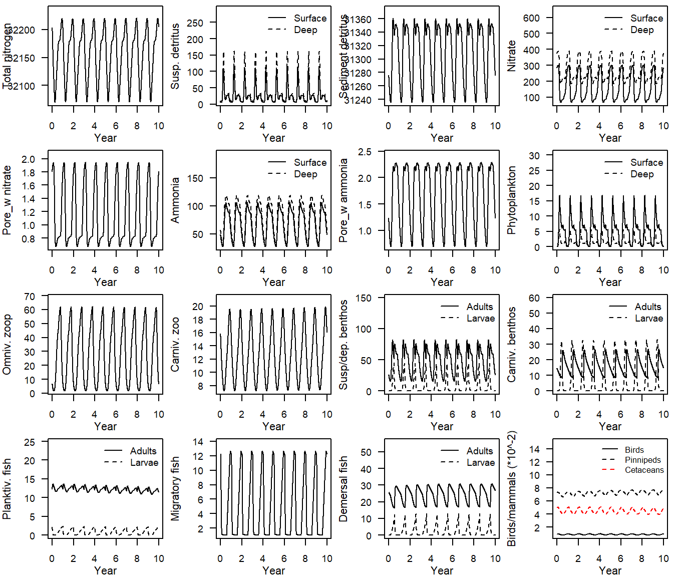
Figure 12. Scenario model run for 2003-2013 in the North Sea with no beam trawlers
It’s hard to see the impacts of the scenario in these basic time series plots, but we can compare the final year annual averaged mass of each food web component using the function e2e_compare_runs_bar() to draw a tornado plot:
mdiff_results <- e2e_compare_runs_bar(selection="AAM",
            model1=NA, use.saved1=FALSE, results1=base_results,
            model2=NA, use.saved2=FALSE, results2=scenario_results,
            log.pc="PC", zone="W",
            bpmin=(-25),bpmax=(+25),
            maintitle="Effect of eliminating beam trawlers")
[1] "Using baseline data held in memory from an existing model run"
[1] "Using scenario data held in memory from an existing model run"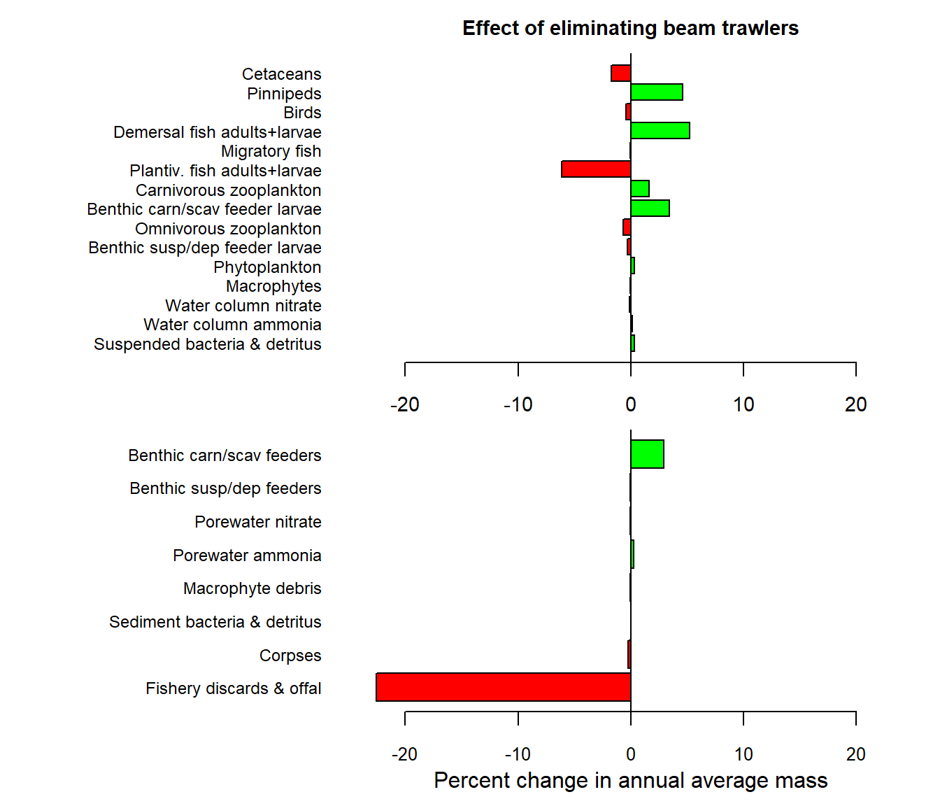
# The dataframe mdiff_results contains the data used in the plot so you can make your own graph if you preferFigure 13. Tornado plot of the percentage different in annual avareged mass of model components between a baseline 2003-2013 model and a scenario in which beam trawling is eliminated. Green bars to the right indicate higher in the scenarion case, red bars to the left indicate less.
Check help(e2e_compare_runs_bar) for options available with this function.